Competitive Equilibrium with Production and Trade
Christopher Makler
Stanford University Department of Economics
(or, Econ 50: Lecture 32)
Econ 51: Lecture 6
pollev.com/chrismakler

Will you need a left-handed desk for exams?
Today's Agenda
- Model 1: Alison and Bob (curved PPFs)
- Incomplete specialization
- Smooth supply and demand curves
- Model 2: Chuck and Wilson (linear PPFs)
- Complete specialization
- Comparative advantage and gains from trade
- Review

You might feel a little like this
by the end of the lecture today.
Don't worry, this is a perfectly natural reaction.
Breathe slowly and deeply, and focus on the economics.
Alison and Bob
Bob's gross demand for good 1 is:
Alison's gross demand for good 1 is:
x_1^B(p_1) = 4 + \tfrac{16}{p_1}
x_1^A(p_1) = 6 + \tfrac{4}{p_1}
p_1
x_1^A
x_1^B
1
10
20
2
8
12
4
7
8
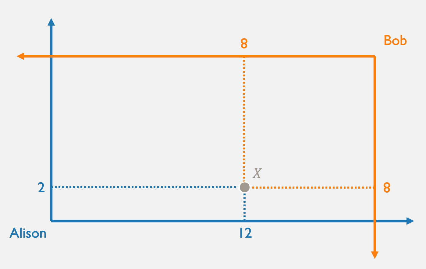
His net demand for good 1 is:
Her net supply of good 1 is:
D_1^B(p_1) = x_1^B(p_1) - 8 = \tfrac{16}{p_1} - 4
S_1^A(p_1) = 12 - x_1^A(p_1) = 6 - \tfrac{4}{p_1}
S_1
2
D_1
12
Bob demands 12
Alison supplies 2
Bob's gross demand for good 1 is:
Alison's gross demand for good 1 is:
x_1^B(p_1) = 4 + \tfrac{16}{p_1}
x_1^A(p_1) = 6 + \tfrac{4}{p_1}
p_1
x_1^A
x_1^B
1
10
20
2
8
12
4
7
8
His net demand for good 1 is:
Her net supply of good 1 is:
D_1^B(p_1) = x_1^B(p_1) - 8 = \tfrac{16}{p_1} - 4
S_1^A(p_1) = 12 - x_1^A(p_1) = 6 - \tfrac{4}{p_1}
S_1
2
D_1
12
Bob demands 4
Alison supplies 4
4
4
Bob's gross demand for good 1 is:
Alison's gross demand for good 1 is:
x_1^B(p_1) = 4 + \tfrac{16}{p_1}
x_1^A(p_1) = 6 + \tfrac{4}{p_1}
p_1
x_1^A
x_1^B
1
10
20
2
8
12
4
7
8
His net demand for good 1 is:
Her net supply of good 1 is:
D_1^B(p_1) = x_1^B(p_1) - 8 = \tfrac{16}{p_1} - 4
S_1^A(p_1) = 12 - x_1^A(p_1) = 6 - \tfrac{4}{p_1}
S_1
2
5
D_1
12
0
(Bob demands 0)
Alison supplies 5
4
4
p_1
1
2
4
Bob's net demand for good 1 is:
Alison's net supply of good 1 is:
D_1^B(p_1) = \tfrac{16}{p_1} - 4
S_1^A(p_1) = 6 - \tfrac{4}{p_1}
S_1
2
5
D_1
12
0
4
4

....but where did this "endowment" come from?
We've been starting with an ‟endowment" of goods...
Step 1: Supply
Joint PPFs with Diminishing MPL
Alison
Bob
MRT = {MP_{L2} \over {MP_{L1}}}=\sqrt{L_1 \over 12L_2}
f_1(L_1) = \sqrt{12L_1}
f_2(L_2) = \sqrt{L_2}
MP_{L1} = \sqrt{3 \over L_1}
MP_{L2} = \sqrt{1 \over 4L_2}
MRT = {MP_{L2} \over {MP_{L1}}}=\sqrt{L_1 \over 2L_2}
f_1(L_1) = \sqrt{12L_1}
f_2(L_2) = \sqrt{6L_2}
MP_{L1} = \sqrt{3 \over L_1}
MP_{L2} = \sqrt{3 \over 2L_2}
Optimal Choice with Prices
Now suppose Chuck can buy and sell these goods at prices \(p_1\) and \(p_2\).
\text{Monetary value of }(y_1,y_2)=p_1y_1 + p_2y_2
Money from spending
another hour producing fish
Money from spending
another hour
producing coconuts
MP_{L1}
\times
p_1
MP_{L2}
\times
p_2
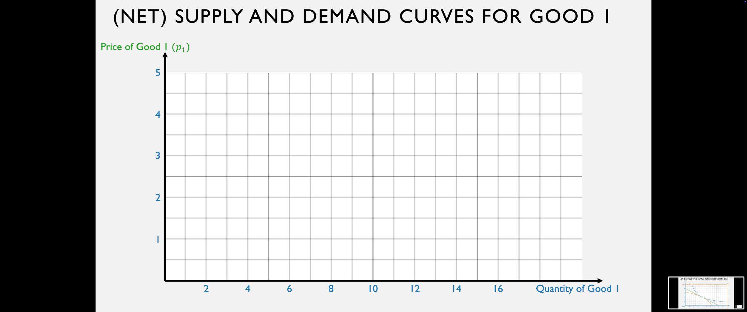
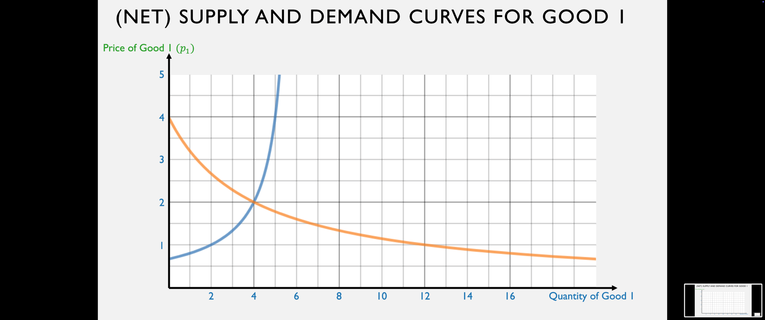
At each price of good 1, we can say how much good 1 each will supply at that price
At each price of good 1, we can say how much good 1 each will supply at that price
Step 2: Demand
y_1^A(p_1,p_2) = \frac{48p_1}{\sqrt{12p_1^2 + p_2^2} }
y_2^A(p_1,p_2) = \frac{4p_2}{\sqrt{12p_1^2 + p_2^2} }
m^A(p_1,p_2) = p_1y_1^A(p_1,p_2) + p_2y_2^A(p_1,p_2)
= p_1 \times \frac{48p_1}{\sqrt{12p_1^2 + p_2^2} } + p_2 \times \frac{4p_2}{\sqrt{12p_1^2 + p_2^2} }
= 4\sqrt{12p_1^2 + p_2^2}
= \frac{48p_1^2 + 4p_2^2}{\sqrt{12p_1^2 + p_2^2} }
Alison's supply decision (which becomes her endowment)
Monetary value of the bundle Alison produces
m^A(p_1,p_2) =
y_1^A(p_1,p_2) = \frac{48p_1}{\sqrt{12p_1^2 + p_2^2} }
y_2^A(p_1,p_2) = \frac{4p_2}{\sqrt{12p_1^2 + p_2^2} }
= 4\sqrt{12p_1^2 + p_2^2}
Alison's supply decision (which becomes her endowment)
Monetary value of the bundle Alison produces
m^A(p_1,p_2) =
Alison's demand for good 1 (if \(u^A(x_1,x_2) = x_1x_2\))
x_1^A(p_1,p_2) = {m^A(p_1,p_2) \over 2p_1}
= \frac{4\sqrt{12p_1^2 + p_2^2} }{2p_1}
=2\sqrt{12 + \left({p_2 \over p_1}\right)^2}
Step 3: Equilibrium
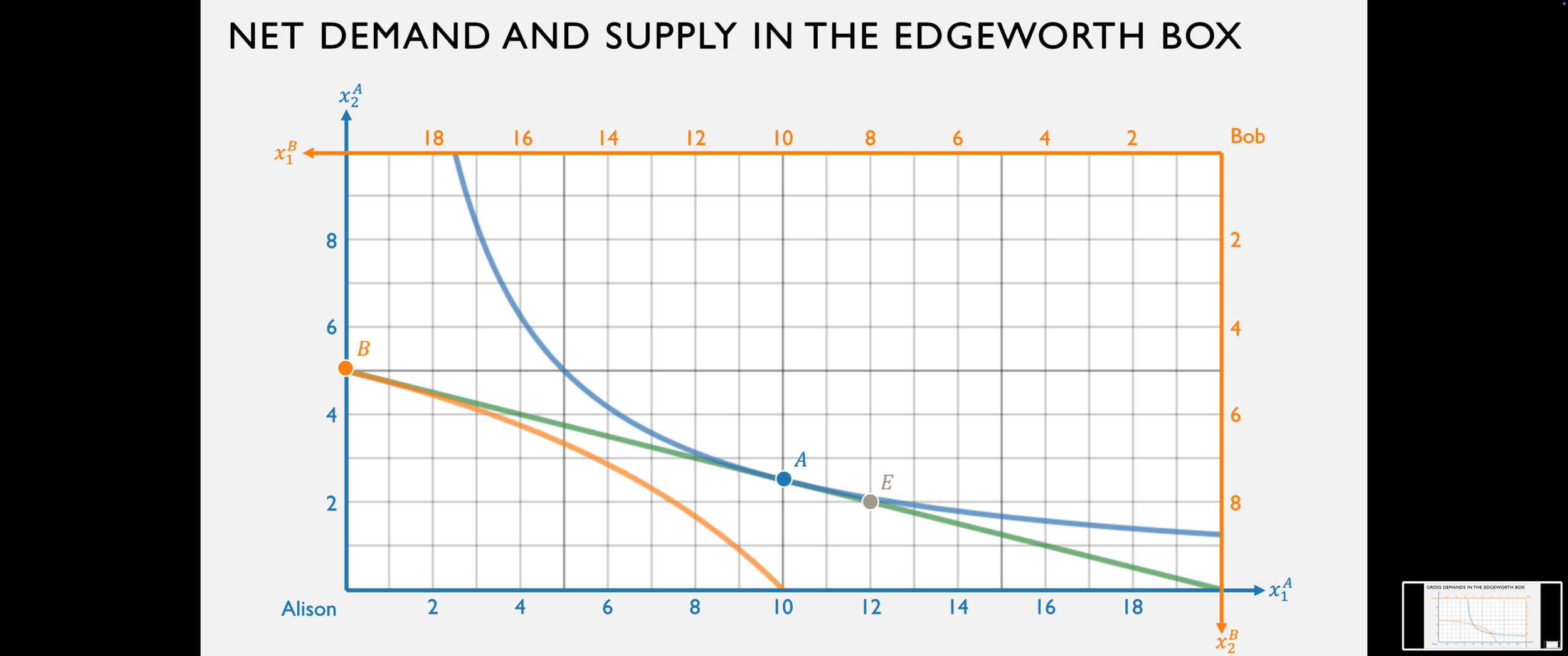
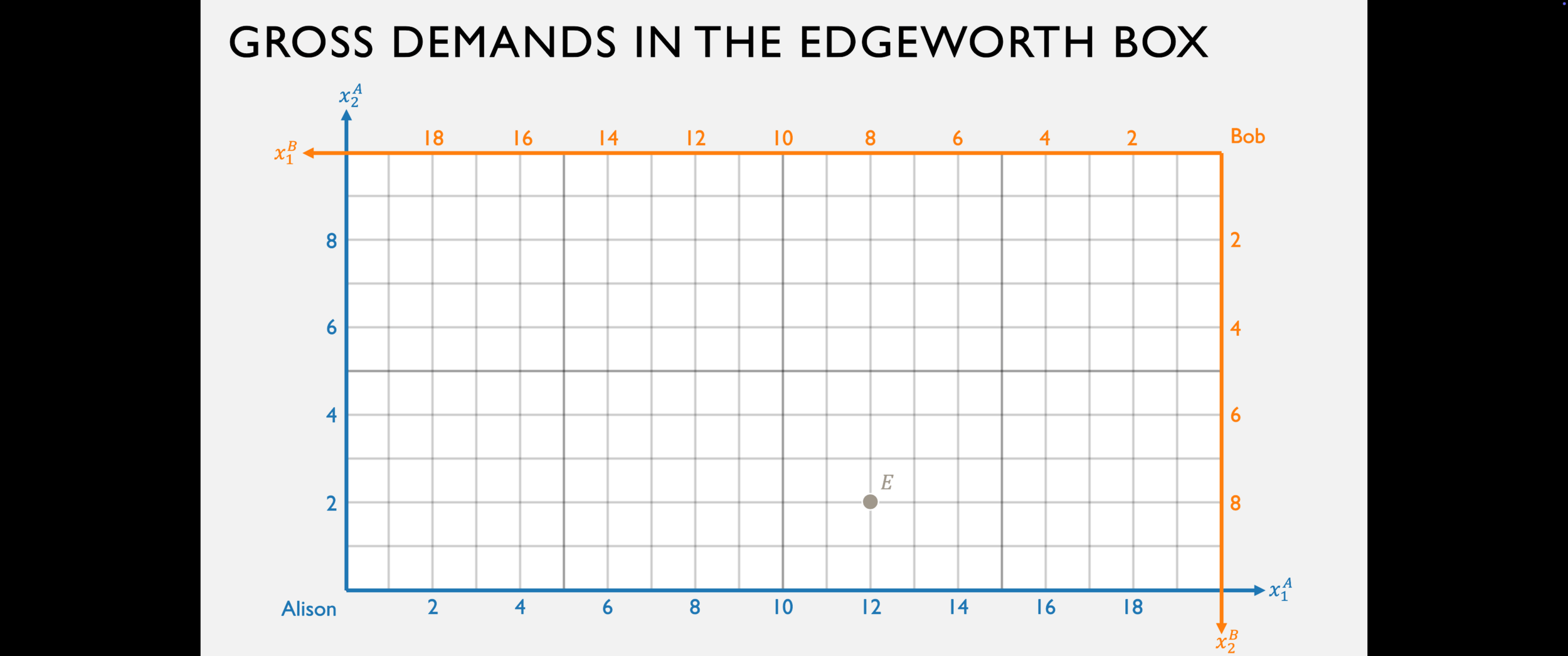
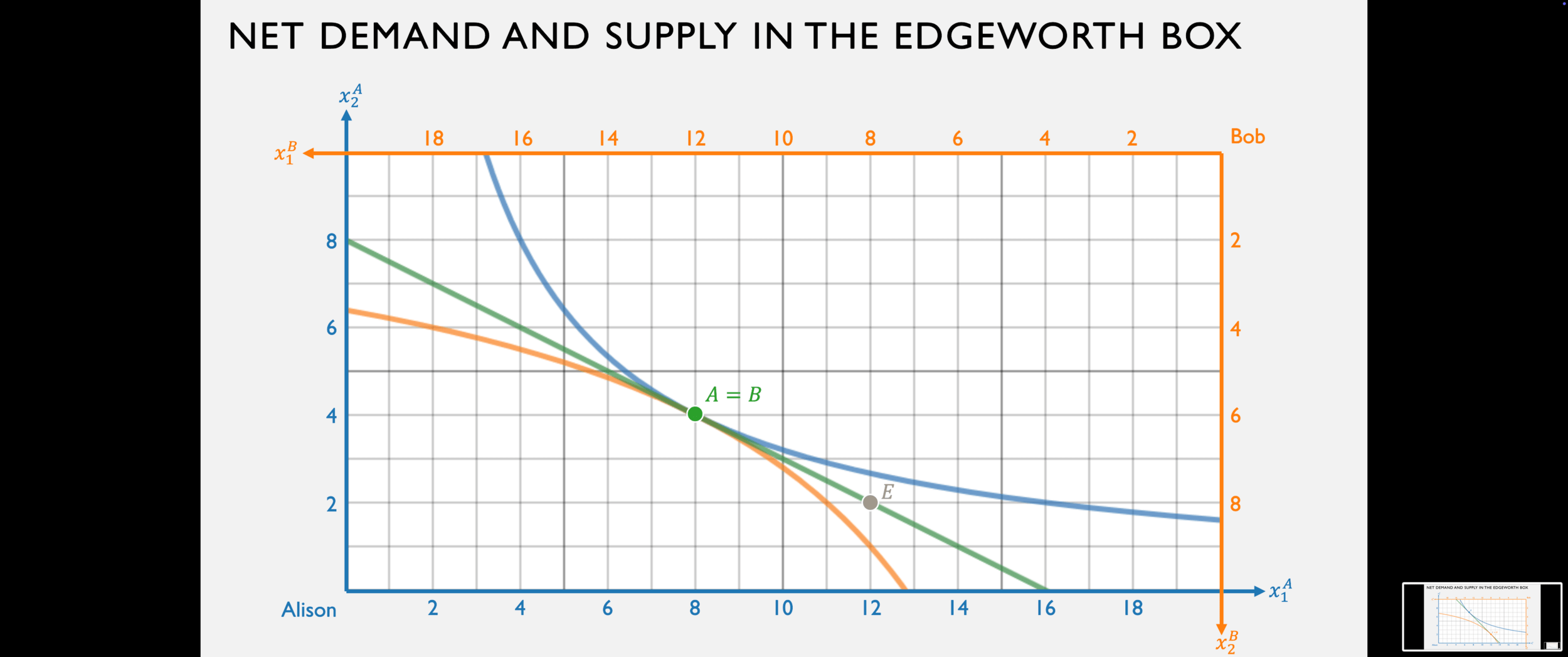
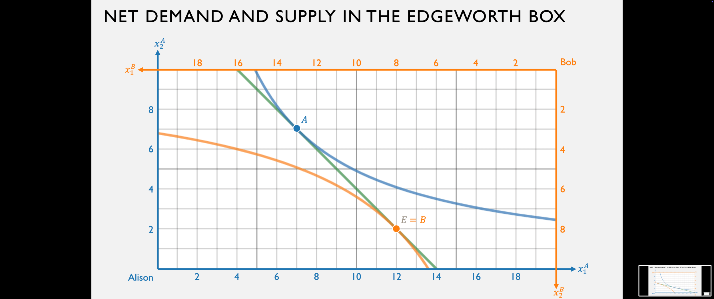
Given any price ratio, Alison and Bob will choose some amounts to produce; this determines the dimensions of the Edgeworth Box, as well as their endowment in it.
They will then choose how much they want to sell of the goods they produced, in order to buy the other good from the other person, at that price ratio.
Competitive equilibrium occurs at the price ratio for which they end up wanting to trade to the same bundle.
Chuck and Wilson
Optimization in Autarky
Marginal Rate of Transformation (MRT)
- The number of coconuts you need to give up in order to get another fish
- Opportunity cost of fish in terms of coconuts
Marginal Rate of Substitution (MRS)
- The number of coconuts you are willing to give up in order to get another fish
- Willingness to "pay" for fish in terms of coconuts
Both of these are measured in
coconuts per fish
(units of good 2/units of good 1)
Marginal Rate of Transformation (MRT)
- The number of coconuts you need to give up in order to get another fish
- Opportunity cost of fish in terms of coconuts
Marginal Rate of Substitution (MRS)
- The number of coconuts you are willing to give up in order to get another fish
- Willingness to "pay" for fish in terms of coconuts
Opportunity cost of marginal fish produced is less than the number of coconuts
you'd be willing to "pay" for a fish.
Opportunity cost of marginal fish produced is more than the number of coconuts
you'd be willing to "pay" for a fish.
Better to spend less time fishing
and more time making coconuts.
Better to spend more time fishing
and less time collecting coconuts.
MRS
>
MRT
MRS
<
MRT
Utility of spending
another hour producing fish
Utility value of spending
another hour producing coconuts
MP_{L1}
=
Optimize by setting them equal to one another
\times
MU_1
MP_{L2}
\times
MU_2
MP_{L1}
=
Optimize by setting them equal to one another
MU_1
MP_{L2}
MU_2
MRS =
= MRT
For a Cobb-Douglas utility function of the form
The “Cobb-Douglas Rule" for Production
u(x_1,x_2) = x_1^ax_2^b
the producer/consumer will optimally spend fraction \(a/(a+b)\) of their total resource value on good 1, and fraction \(b/(a+b)\) on good 2.
Example: Chuck has 12 hours of labor, and can produce 2 coconuts per hour or 1 fish per hour.
His preferences may be represented by the utility function \(u(x_1,x_2) = x_1x_2^2\)
What does the Cobb-Douglas rule say he should do?
Specialization and Trade
Now suppose Chuck can buy and sell these goods at prices \(p_1\) and \(p_2\).
\text{Monetary value of }(y_1,y_2)=p_1y_1 + p_2y_2
Notation: \(y_i\) is the amount he produces of good \(i\); \(x_i\) is the amount he consumes.
Money from spending
another hour producing fish
Money from spending
another hour
producing coconuts
MP_{L1}
\times
p_1
MP_{L2}
\times
p_2
With linear production functions, he should completely specialize in one or the other!
Two Agents
Solving for Equilibrium I: Production
We know that Chuck and Wilson have different opportunity costs of producing fish:
MRT = {1 \over 2}
CHUCK
MRT = 1
WILSON
For what range of price ratios will each of them specialize in the good for which they have a comparative advantage?
Solving for Equilibrium II: Trade
Once everyone is specializing, we have the endowments:
(24,0)
CHUCK
(0,36)
WILSON
How much fish will each supply and demand at different prices?
u(x_1,x_2) = x_1x_2^2
Suppose both Chuck and Wilson have
Cobb-Douglas preferences given by
(24,0)
CHUCK
(0,36)
WILSON
u(x_1,x_2) = x_1x_2^2
Let's fix \(p_2 = 1\) and solve for \(p_1\).
VALUE OF ENDOWMENT
\hat m^A = 24p_1
\hat m^B = 36
OPTIMAL CHOICE
x_1^A = 8
x_1^B = {12 \over p_1}
x_1^* = {\hat m \over 3p_1}
SUPPLY AND DEMAND
s_1^A(p_1) = 16
d_1^B(p_1) = {12 \over p_1}
p_1^* = {3 \over 4}
What have we learned?
Far out in the uncharted backwaters of the unfashionable end of the western spiral arm of the Galaxy lies a small unregarded yellow sun.

SCIEPRO/GETTY IMAGES
Orbiting this at a distance of roughly ninety-two million miles is an utterly insignificant little blue green planet whose ape-descended life forms are so amazingly primitive that they still think digital watches are a pretty neat idea.
This planet has — or rather had —
a problem, which was this:
😢
most of the people on it were unhappy for pretty much of the time.
Many solutions were proposed
for this problem...
...but most of these were largely concerned with the movements
of small green pieces of paper,
which is odd because on the whole
it wasn't the small green pieces of paper that were unhappy.

Resources
Technology
Stuff
Happiness
🌎
🏭
⌚️
🤓
The Real World
Demand
Supply
Equilibrium
🤩
🏪
⚖
Little Green
Pieces of Paper
Resources
Technology
Stuff
Happiness
🌎
🏭
⌚️
🤓
The Real World

Little Green
Pieces of Paper
- A change in the price of a good results in a movement along its demand curve
- A change in income or the price of other goods results in a shift of the demand curve
f(L,K) = \sqrt{LK}, \overline K = 32
64 + {1 \over 4}q^2
{1 \over 2}q
pq
\pi(q) = \ \ \ \ \ - [\ \ \ \ \ \ \ \ \ \ \ \ \ \ \ ]
\pi^\prime(q) = \ \ \ - \ \ \ \ \ \ \ \ = 0
p
TR
TC
MR
MC
Take derivative and set = 0:
Solve for \(q^*\):
q^*(p) = 2p
SUPPLY FUNCTION
"Keep producing output as long as the marginal revenue from the last unit produced is at least as great as the marginal cost of producing it."
"Keep hiring workers as long as the marginal revenue from the output of the last worker is at least as great as the cost of hiring them."
p = MC
w = MRP_L
Profit as a function of output \(q\)
Profit as a function of labor \(L\)
p = w \times {1 \over MP_L}
w = p \times MP_L
So...how do firms choose a point along the PPF?
Consider a PPF with "guns" (military goods) and "butter" (civilian goods)
An international conflict increases the demand for guns. What effect does this have on the market for butter?
Step 1: The increased demand for guns raises the price of guns, thereby increasing the demand for labor by gun firms at every wage:
So, let's put this all together.
The increase in demand for guns leads to an increase in overall labor demanded, which leads to an increase in the wage rate.
What effect does this have on the supply curves of guns and butter?
Conditions for
GDP Maximization
{p_1 \over p_2} = MRT
TANGENCY CONDITION
CONSTRAINT CONDITION
L_1(Y_1) + L_2(Y_2) = \overline L
Firms in industry 1 set \(w = p_1 \times MP_{L1}\)
Firms in industry 2 set \(w = p_2 \times MP_{L2}\)
How does competition achieve this?
Wages adjust until the
labor market clears

General Equilibrium
The Circular Flow
In our consumer theory, we've treated income as exogenous.
In our producer theory, we've treated wages as exogenous.
We've also assumed firms are maximizing profits, but haven't said where those profits go.
Crazy thought: what if the money firms pay for labor becomes the income of workers?
...and their profits become the income of the owners/shareholders of the firm?
Consumers
Good 1 Firms
Market for Good 1
Market for Good 2
Market for Labor
Good 2 Firms
Money flows clockwise
Goods, labor flow counter-clockwise
General Equilibrium: Everyone optimizes, all markets clear simultaneously.
Competitive Equilibrium
We sometimes call the autarky model the "centralized" model: if there were a single agent making a decision, what would they do?
Similarly, we call competitive equilibrium a "decentralized" model, because lots and lots of individuals are making small decisions that add up to what "society chooses"
1. Given prices \(p_1,p_2\), firms will choose the point \((Y_1^*,Y_2^*)\) along the PPF where \(MRT = \frac{p_1}{p_2}\)
2. All money received by firms \((p_1Y_1^* + p_2Y_2^*)\) will become income \(M\) for consumers.
3. Given prices \(p_1,p_2\) and income \(M\), the consumer will choose the point \((X_1^*,X_2^*)\) along the budget line where \(MRS = \frac{p_1}{p_2}\)
4. At equilibrium prices, markets clear (\(X_1^* = Y_1^*\) and \(X_2^* = Y_2^*\)) so \(MRS = MRT\).
5. In disequilibrium, there is a shortage in one market and a surplus in the other, pulling the system toward equilibrium.
Overview of General Equilibrium
1. Given prices \(p_1,p_2\), firms will choose the point \((Y_1^*,Y_2^*)\) along the PPF where \(MRT = \frac{p_1}{p_2}\)
2. All money received by firms \((p_1Y_1^* + p_2Y_2^*)\) will become income \(M\) for consumers.
3. Given prices \(p_1,p_2\) and income \(M\), consumers will choose the point \((X_1^*,X_2^*)\) along the budget line where \(MRS = \frac{p_1}{p_2}\)
MRS =
p_1
p_2
= MRT
If consumers and firms all face the same price, and if they choose the same quantity in response to that price, then MRS = MRT.
The Neoclassical Model
If every decision involves setting the marginal cost of any decision equal to the marginal benefit
(or the marginal opportunity cost equal to the marginal rate of substitution), AND
if everyone bases their decisions on a common price (either for selling or buying each good), THEN
prices in perfectly competitive markets act as a coordination mechanism that equates
one person's marginal cost to another's marginal benefit
THE INVISIBLE HAND IS MAGIC
FREE MARKETS ARE EFFICIENT
There's just one tiny problem...
That's not the world we live in.
Next 7 weeks: it all falls apart.
Econ 50 | 06 | The Neoclassical Model
By Chris Makler
Econ 50 | 06 | The Neoclassical Model
General equilibrium


