Cost Curves
To navigate: press "N" to move forward and "P" to move back.
To see an outline, press "ESC". Topics are arranged in columns.
Cost Curvature
To navigate: press "N" to move forward and "P" to move back.
To see an outline, press "ESC". Topics are arranged in columns.
Unit Overview: Profit Maximization
Cost Curves
("Technology" and "Cost Curves" chapters)
Competitive Supply
("Firm Supply" and "Industry Supply" Chapters)
Market Power
("Monopoly" Chapter)
Given a cost function c(y) and demand conditions, what is the profit-maximizing quantity y*?
Input Demands
("Profit Maximization" Chapter)
Note: Usually we will just assign
selections from these chapters.
Specific sections will be indicated in the quiz.
Don't read the whole chapters!!
Today's Agenda
Hour 1: Total and Unit Cost Curves
Hour 2: Relationship of Production to Cost
Review: Expansion paths and total cost
Fixed and variable costs
Average costs
Marginal cost
Relationship between Average & Marginal
Production and Cost with One Input
Returns to Scale with Two Inputs
Economies and Diseconomies of scale
Review: Expansion Paths and
Short-Run and Long-Run Total Costs
\text{Ongoing Mathematical Example: }f(L,K) = L^\frac{1}{4} K^\frac{1}{4}
c(w,r,y) = 2\sqrt{wr}y^2
c_s(w,r,y) = w\frac{y^4}{\overline{K}} + r\overline{K}
\text{Last time we found the LR and SR total cost functions: }
\text{Now let's fix }w=r=10\text{ and }\overline K = 25:
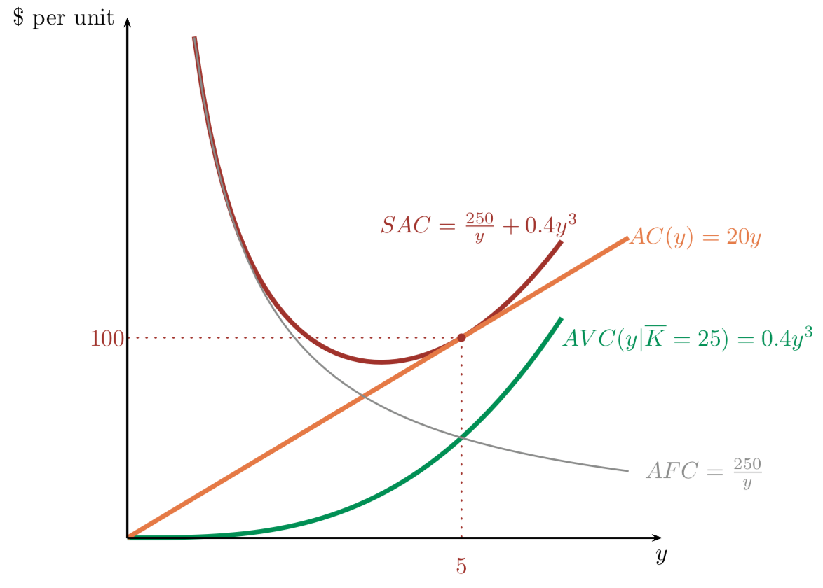
c(y) = 20y^2
c_s(y) = 250+0.4y^4
LONG RUN
SHORT RUN
Fixed and Variable Costs
Fixed and Variable costs
c_s(y,\overline{K}) = wL(y,\overline{K}) + r\overline{K}
Cost of variable inputs
Cost of fixed inputs
c(y) = c_v(y) + F
From input decision ("Cost Minimization" chapter):
When thinking about output ("Cost Curves" chapter):
Fixed Costs (F): All economic costs that don't vary with output.
Variable Costs (VC): All economic costs that vary with output
Opp. costs, sunk costs, "quasi-fixed" costs
\text{Ongoing Mathematical Example: }f(L,K) = L^\frac{1}{4} K^\frac{1}{4}
c(y) = 20y^2
c_s(y) = 250+0.4y^4
LONG RUN
SHORT RUN
F
c_v(y)

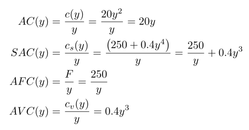
Average Costs
\text{Total Cost (TC)}: c(y) = c_v(y) + F
\text{Average Cost (AC)}: \frac{c(y)}{y} = \frac{c_v(y)}{y} + \frac{F}{y}
Fixed Costs (F)
Variable Costs (VC)
Average Fixed Costs (AFC)
Average Variable Costs (VC)
Average fixed, variable, and total costs

c(y) = 20y^2
c_s(y) = 250+0.4y^4
LONG RUN
SHORT RUN
\text{Ongoing Mathematical Example: }f(L,K) = L^\frac{1}{4} K^\frac{1}{4}
Comparing Total and Average Costs
Fixed costs are constant;
average fixed costs start at infinity and decrease
Variable costs start from zero and increase;
so do average variable costs.
Short-run total costs start at F and increase by VC;
SAC start out like AFC (since AVC = 0) and end up like AVC (as AFC approaches 0).
Long-run total costs start from zero and increase;
so do long-run average total costs.
This is because we're assuming there are no other fixed costs (e.g. opp. costs)
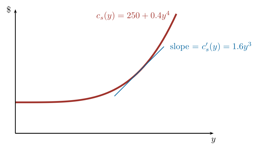
Marginal Costs
\text{Total Cost (TC)}: c(y) = c_v(y) + F
\text{Marginal Cost (MC)}: c'(y) = c_v'(y) + 0
Fixed Costs (F)
Variable Costs (VC)
(Marginal cost = marginal variable cost)
c(y) = 20y^2
c_s(y) = 250+0.4y^4
LONG RUN
SHORT RUN
LMC(y) = c'(y) = 40y
SMC(y) = c'_s(y) = 1.6y^3
\text{Ongoing Mathematical Example: }f(L,K) = L^\frac{1}{4} K^\frac{1}{4}
Relationship between Average and Marginal Costs
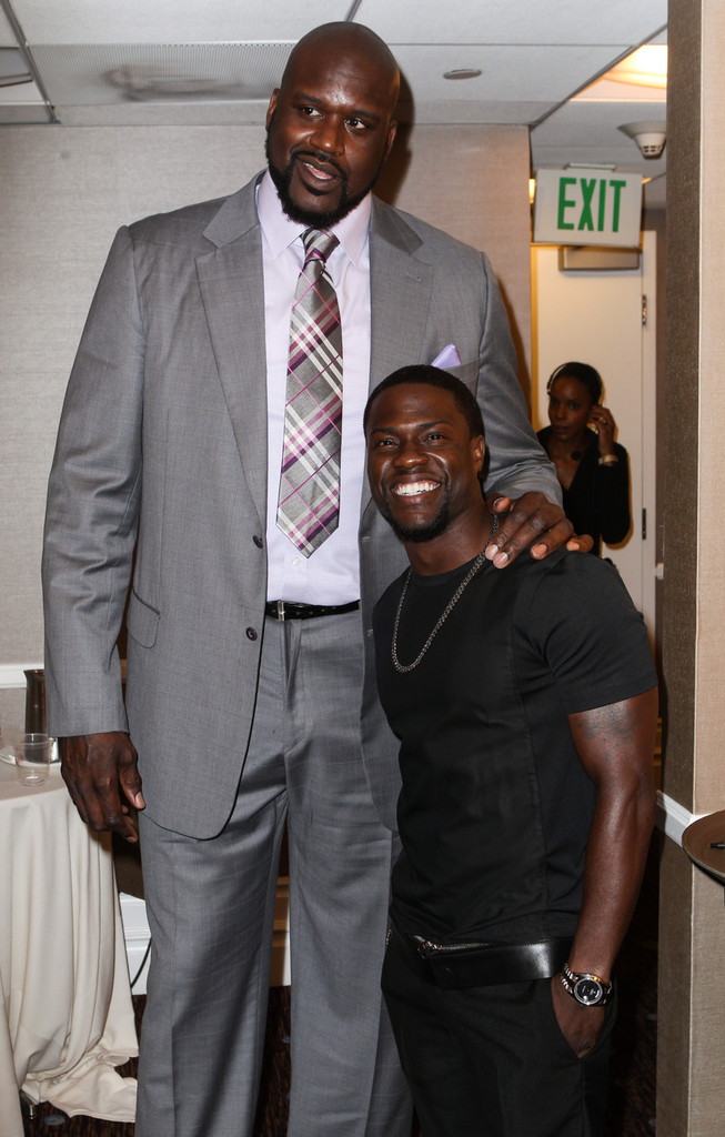
Shaquille O'Neal is 7'1" (216cm)
Kevin Hart is 5'4" (163cm)
What would happen to the average height in this room if Shaquille O'Neal walked in?
What about if Kevin Hart walked in?
Marginal cost tends to “pull" average cost toward it:
MC > AC \Rightarrow AC \text{ increasing}
MC = AC \Rightarrow AC \text{ constant}
MC < AC \Rightarrow AC \text{ decreasing}
Marginal grade = grade on last test, average grade = GPA
\text{Ongoing Mathematical Example: }f(L,K) = L^\frac{1}{4} K^\frac{1}{4}
c_s(y) = 250+0.4y^4
SHORT RUN
SMC(y) = c'_s(y) = 1.6y^3
SAC(y) = \frac{c_s(y)}{y} = \frac{250}{y} + 0.4y^3


[10 minute break]
Production and Cost with One Input
The Nature of the Production Function affects the Curvature of the Total Cost Curve.
Decreasing marginal returns => increasing marginal cost
Constant marginal returns => constant marginal cost
Increasing marginal returns => decreasing marginal cost
This is going to be true in different ways as we shift to two inputs...
Returns to Scale in the Long Run
Returns to a Single Input
- Increasing marginal product: MPL is increasing in L
- Constant marginal product: MPL is constant in L
- Diminishing marginal product: MPL is decreasing in L
Returns to Scale (Scaling all inputs.)
- Increasing returns to scale: doubling all inputs more than doubles output.
- Constant returns to scale: doubling all inputs exactly doubles output.
- Decreasing returns to scale: doubling all inputs less than doubles output.

Original
Double width
Double both
How do the attributes of the production function
(diminishing marginal product, returns to scale)
affect average costs?
Intuitively: if you have diminishing productivity,
you'll have increasing marginal costs
and eventually increasing average costs.
Relationship between Production Function and the Curvature of Long-Run and Short-Run Costs
- If the production function has diminishing \(MP_L\), the short-run cost curve will get steeper as you produce more output (have increasing marginal costs)
- If the production function has decreasing returns to scale, the long-run cost curve will get steeper as you produce more output.
- What about for constant returns to scale? Increasing returns to scale?
Economies and Diseconomies of Scale
Returns to Scale
Has to do with the production function
Economies of Scale
Has to do with cost curves
Increasing Returns to Scale:
double input => more than double output
Decreasing Returns to Scale:
double input => less than double output
Always deals with the long run
Can occur in both the long run and short run
Economies of Scale:
increasing output lowers average costs
Diseconomies of Scale:
increasing output raises average costs
Last time we derived the short-run and long-run total cost curves as the result of a cost-minimization problem.
Unit costs (average costs and marginal costs) are direct derivations from the total cost functions.
The curvature of cost curves is related to the nature of the production function: diseconomies of scale and rising marginal costs come from diminishing marginal returns to inputs.
Conclusion and Next Steps
Next week: profit maximization for competitive firms, then with market power...
Econ 50 | 11 | Cost Curves (Shriram)
By Chris Makler
Econ 50 | 11 | Cost Curves (Shriram)
Having derived the total cost of producing y units in the short run and long run, we take a closer look at total cost (fixed and variable) and unit cost curves (average and marginal). We then examine the relationship between the nature of production processes and their associated cost curves.


