


Content ITV PRO
This is Itvedant Content department
Learning Outcome
5
Reverse the scaling to interpret predictions in real dollar values
4
Train (fit) the model on your prepared 3D data
3
Compile the model with the correct optimizer and loss function
2
Add an LSTM layer configured for time series data
1
Build a Sequential neural network architecture in Keras
Theory & Scaling
Scaled data between 0 and 1 (MinMax)
60-Day Slicing
Lookback windows created
3D Reshape
Tensor shape: (Samples, 60, 1)
Fueling
THE ENGINE
Keras LSTM Model
Ready to Build
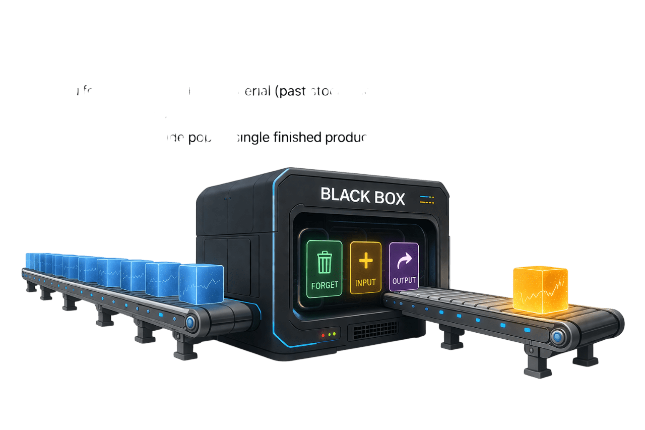
Think of the LSTM as a highly advanced factory machine
You feed it 60 days of raw material (past stock prices).
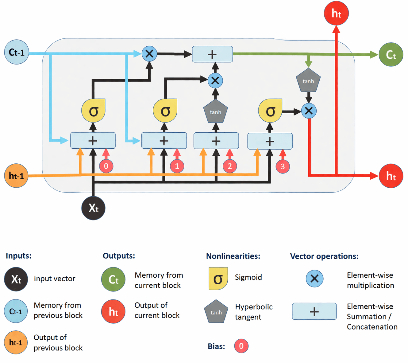
Inside the "Black Box," the Forget, Input, and Output gates process the patterns.
Out of the other side pops a single finished product: Tomorrow's Price.
Tomorrow's Price
60 Days of Stock Prices
Today, we write the Python code to build this exact machine
Step 1
Every great structure starts with a foundation.
We begin by creating a blank linear stack of layers.
# Import the building blocks
from tensorflow.keras.models import Sequential
from tensorflow.keras.layers import LSTM, Dense

# Initialize the blank canvas
model = Sequential()

# The model is currently empty
# Waiting for layers to be added...Step 2
# Add the LSTM Layer
model.add(LSTM(
    units=50,
        # Number of memory cells
    input_shape=(X_train.shape[1], 1)
 # 60 time steps, 1 feature
))

# "units=50" gives the model 50 neurons
# "input_shape" defines the 3D tensor
Adding the intelligence to process time-series patterns.
50 memory cell
60 Times step
Step 3
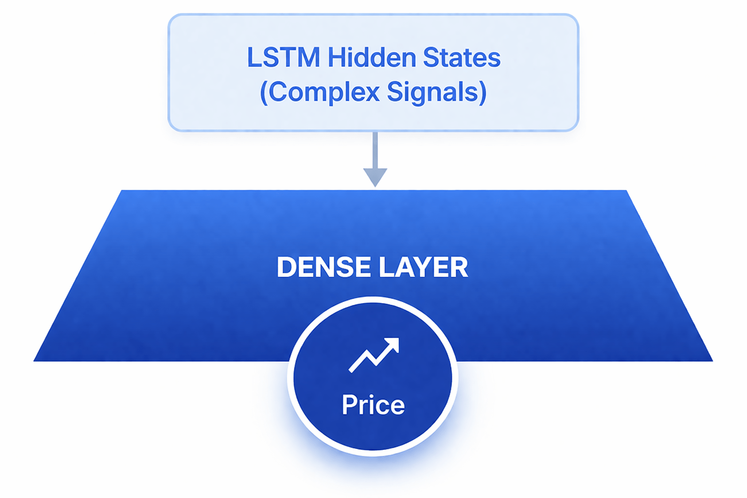
# Add the Output Layer
model.add(
Dense(units=1)
)

# We need a single numerical output
# units=1 signifies one final prediction
# Tomorrow's Stock Price
Step 4
optimizer='adam'
The smart driver that adjusts weights to minimize errors.
loss='mse'
The scoring system (Mean Squared Error). Target is zero.
# Set the rules for learning
model.compile(
    optimizer='adam',
            # The smart driver
    loss='mean_squared_error'
    # The scoring system
)

# Optimizer: Adam adjusts learning rate automatically
# Loss: MSE measures the average squared difference
Step 5
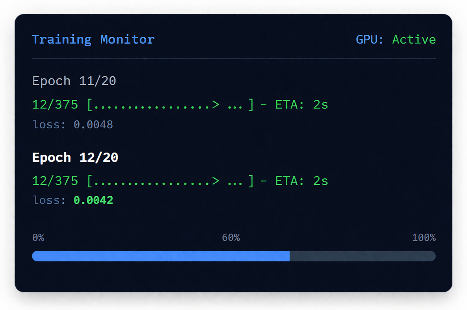
# Feed data and start learning
model.fit(
    X_train,
    y_train,
    epochs=20,
        # Full passes through data
    batch_size=32
   # Samples per gradient update
)

# Epochs: Model reads dataset 20 times
# Batch Size: Updates weights every 32 windows
Now we feed our 3D data into the model and let it learn!
Step 6
# Feed unseen test data to model
predictions =
model.predict(X_test)
# Let's inspect the first prediction
print(predictions[0])
# Output:
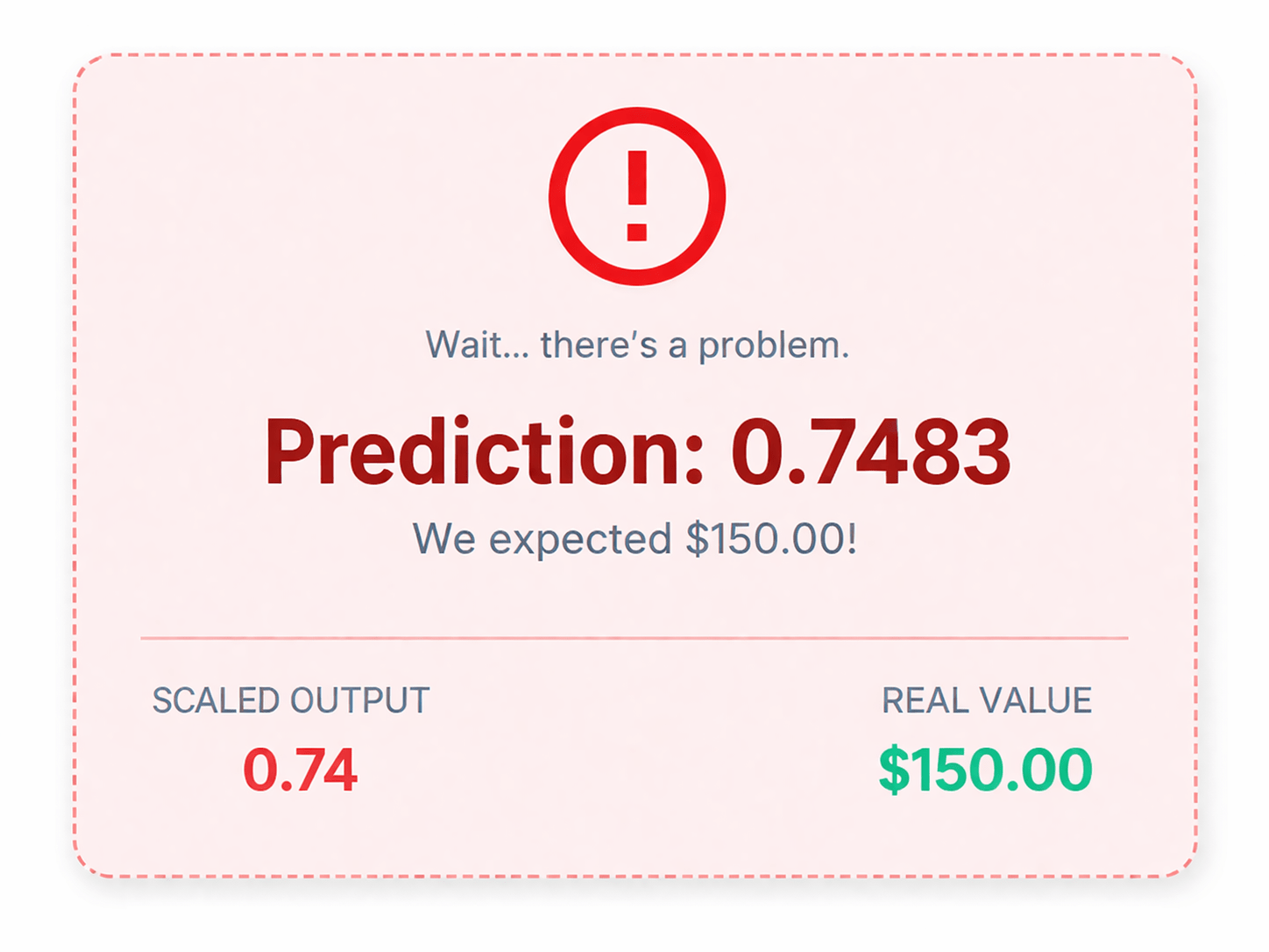
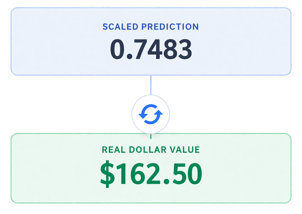
# [0.7483322]Step 7
# Reverse the scaling process!
real_predictions =
scaler.inverse_transform(predictions)


# The model output was squashed (0-1)
# This stretches it back to reality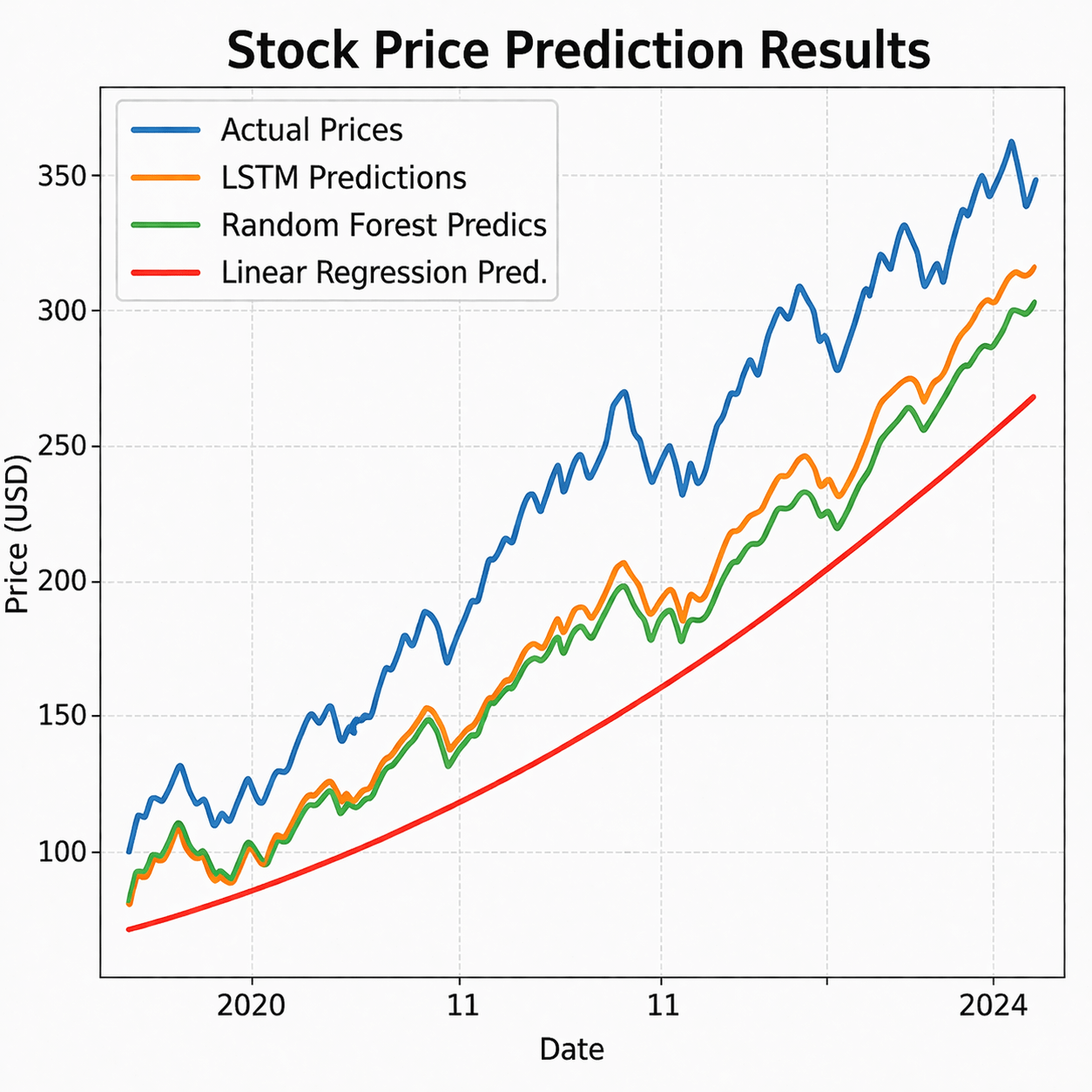
# 0.81 ➔ $162.50Overlaying our predictions on real-world stock prices reveals how closely the LSTM learned the underlying trend.
Summary
5
6
.fit() the model on the training data.
.fit() the model on the training data.
.predict() the test data and apply inverse_transform().
4
.compile() with Adam optimizer and MSE loss.
3
Add Dense(1) layer for the final output.
2
Add LSTM() layer with correct input_shape.
1
Initialize Sequential() model.
Quiz
Why do we add a Dense(units=1) layer at the very end of our LSTM network for stock prediction?
A) To increase the memory of the LSTM
B) To output a single continuous value (the predicted price)
C) To convert the data into a 3D tensor
D) To scale the data between 0 and 1
Quiz-Answer
Why do we add a Dense(units=1) layer at the very end of our LSTM network for stock prediction?
A) To increase the memory of the LSTM
B) To output a single continuous value (the predicted price)
C) To convert the data into a 3D tensor
D) To scale the data between 0 and 1
By Content ITV


