Deep Learning
- Crash Course -
UNIFEI - August, 2018
Hello!
Prof. Luiz Eduardo
Hanneli Tavante


<3
Canada
Prof. Maurilio

<3
Deutschland
Questions
- What is this course?
- A: An attempt to bring interesting subjects to the courses
- Why are the slides in English?
- I am reusing some material that I prepared before
- What should I expect?
- This is the first time we give this course. We will be looking forward to hearing your feedback
Rules
- Don't skip classes
- The final assignment is optional
- We will have AN OPTIONAL LECTURE on Friday
- Feel free to ask questions
- Don't feel discouraged with the mathematics
- Contact us for study group options
[GIF time]

Agenda
- Why is deep learning so popular now?
- Introduction to Machine Learning
- Introduction to Neural Networks
- Deep Neural Networks
- Training and measuring the performance of the N.N.
- Regularization
- Creating Deep Learning Projects
- CNNs and RNNs
- (OPTIONAL): Tensorflow intro
Note: this list can change
Topics
- Why is deep learning so popular now?
- Introduction to Machine Learning
- Introduction to Neural Networks
- Deep Neural Networks
- Training and measuring the performance of the N.N.
- Regularization
- Creating Deep Learning Projects
- CNNs and RNNs
- (OPTIONAL): Tensorflow intro
Note: this list can change
What is the difference between Machine Learning (ML) and Deep Learning (DL)? And AI?
AI
ML
Representation Learning
DL
Why is it so popular?
- Big companies are using it
- Business opportunities
- It is easy to understand the main idea
- More accessible outside the Academia
- Lots os commercial applications
- Large amount of data
- GPUs and fast computers
Agenda
- Why is deep learning so popular now?
- Introduction to Machine Learning
- Introduction to Neural Networks
- Deep Neural Networks
- Training and measuring the performance of the N.N.
- Regularization
- Creating Deep Learning Projects
- CNNs and RNNs
- (OPTIONAL): Tensorflow intro

WHERE ARE THE
NEURAL
NETWORKS??////??
<3
Canada
Agenda
- Why is deep learning so popular now?
- Introduction to Machine Learning (we are still here)
- Introduction to Neural Networks
- Deep Neural Networks
- Training and measuring the performance of the N.N.
- Regularization
- Creating Deep Learning Projects
- CNNs and RNNs
- (OPTIONAL): Tensorflow intro
Example: predict if a given image is the picture of a dog
Our Data and Notation
(x, y) ; x \in \mathbb{R}^n;
y \in {0, 1}
Let us use the Logistic Regression example
Single training example
We will have multiple training examples:
m training examples in a set
{ (x^{(1)}, y^{(1)}), (x^{(2)}, y^{(2)}), ..., (x^{(m)}, y^{(m)})}
Warning:
( [
x^{(1)}_1
],
x^{(1)}_2
| First x vector | First y (number) |
|---|---|
| Second x vector | Second y (number) |
| ... | ... |
x^{(1)}_3
x^{(1)}_4
y^{(1)}
)
Warning:
( [
x^{(1)}_1
],
x^{(1)}_2
| First x vector | First y (number) |
|---|---|
| Second x vector | Second y (number) |
| ... | ... |
x^{(1)}_3
x^{(1)}_4
y^{(1)}
)
( [
x^{(2)}_1
],
x^{(2)}_2
x^{(2)}_3
x^{(2)}_4
y^{(2)}
)
Pro tip:
[
x^{(1)}_1
x^{(1)}_2
| First x vector | First y (number) |
|---|---|
| Second x vector | Second y (number) |
| ... | ... |
x^{(1)}_3
x^{(1)}_4
x^{(2)}_1
...]
x^{(2)}_2
x^{(2)}_3
x^{(2)}_4
m
n
Pro tip:
[
x^{(1)}_1
x^{(1)}_2
| First x vector | First y (number) |
|---|---|
| Second x vector | Second y (number) |
| ... | ... |
x^{(1)}_3
x^{(1)}_4
x^{(2)}_1
...]
x^{(2)}_2
x^{(2)}_3
x^{(2)}_4
m
n
[
y^{(1)}
y^{(2)}
...]
Data:
| [salary, location, tech...] | Probability y=1 |
|---|---|
| [RGB values] | 0.8353213 |
| ... | ... |
In logistic regression, we want to know the probability of y=1 given a vector of x
\hat{y} = P(y=1 | x)
(note: we could have more columns for extra features)
Logistic regression
Recap: for logistic regression, what is the equation format?
Tip: Sigmoid, transpose, wx+b
w_1
w_2
w_3
x_1
x_2
x_3
*

Logistic regression
Recap: for logistic regression, what is the equation format?
Tip: Sigmoid, transpose, wx+b
w_1
w_2
w_3
x_1
x_2
x_3
*
+
b
z
Logistic regression
Recap: for logistic regression, what is the equation format?
Tip: Sigmoid, transpose, wx+b
w_1
w_2
w_3
x_1
x_2
x_3
*
+
b
z
\hat{y} = \sigma
(
)
\sigma=\frac{1}{1+e^{-z}}
Logistic regression
Recap: given a training set
{ (x^{(1)}, y^{(1)}), (x^{(2)}, y^{(2)}), ..., (x^{(m)}, y^{(m)})}
You want
\hat{y}^{i} \approx y^i
What do we do now?
loss = -y \log(h(x)) - (1-y)\log(1 - h(x))
For each training example
Logistic regression
L(\hat{y}, y) = -y \log(\hat{y}) - (1-y)\log(1 - \hat{y})
For each training example
If y = 1, you want
\hat{y}
large
If y = 0, you want
\hat{y}
small
What do we do now?
Cost function: applies the loss function to the entire training set
J(w, b) = \frac{1}{m} \sum_{i=1}^{m} [L(\hat{y}, y) ]
Logistic regression
What do we do now?
Cost function: measures how well your parameters are doing in the training set
J(w, b) = \frac{1}{m} \sum_{i=1}^{m} [L(\hat{y}, y) ]
We want to find w and b that minimise J(w, b)
Gradient Descent: it points downhill
It's time for the partial derivatives
Logistic regression
J(w, b) = \frac{1}{m} \sum_{i=1}^{m} [L(\hat{y}, y) ]
Gradient Descent: It's time for the partial derivatives
source: https://www.wikihow.com/Take-Derivatives
Logistic regression
J(w, b) = \frac{1}{m} \sum_{i=1}^{m} [L(\hat{y}, y) ]
We are looking at the previous step to calculate the derivative
source: https://www.wikihow.com/Take-Derivatives
Whiteboard time - computation graphs and derivatives
Let's put these concepts together
x
w
b
z=w^T+b
\hat{y} = a = \sigma(z)
L(\hat{y}, y) = L(a, y)
Forward pass
What is our goal?
Adjust the values of w and b in order to MINIMIZE difference at the loss function
x
w
b
z=w^T+b
\hat{y} = a = \sigma(z)
L(\hat{y}, y) = L(a, y)
How do we compute the derivative?
The equations: (whiteboard)
Backwards step
x
w
b
z=w^T+b
\hat{y} = a = \sigma(z)
L(\hat{y}, y) = L(a, y)
Good news: this looks like a Neural Network!
Agenda
- Why is deep learning so popular now?
- Introduction to Machine Learning
- Introduction to Neural Networks
- Deep Neural Networks
- Training and measuring the performance of the N.N.
- Regularization
- Creating Deep Learning Projects
- CNNs and RNNs
- (OPTIONAL): Tensorflow intro

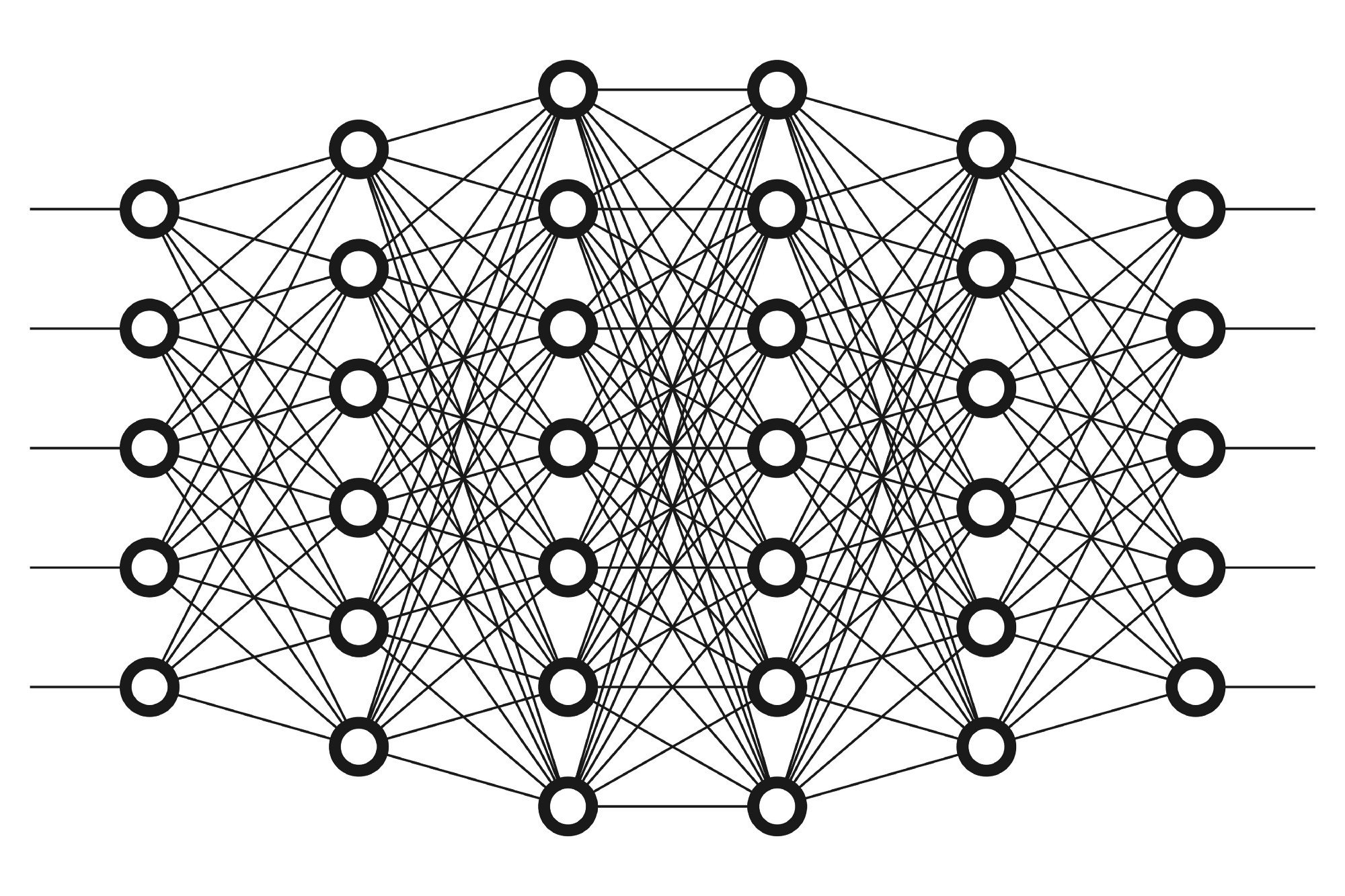
Basic structure of a Neural Network
x_1
x_2
x_3
Hidden
Layer
\hat{y}
More details
x_1
x_2
x_3
Hidden Layer
\hat{y}
Hidden Layer
In each hidden unit of each layer, a computation happens. For example:
z=w^T+b
a = \sigma(z)
Naming convention
x_1
x_2
x_3
Hidden Layer
\hat{y}
Hidden Layer
a^{[1]}
a^{[1]}_1
a^{[1]}_3
a^{[1]}_2
a^{[2]}
a^{[2]}_1
a^{[1]} = [a^{[1]}_1, a^{[1]}_2, a^{[1]}_3]
a^{[2]} = \hat{y}
X = a^{[0
]}
Key question: Every time we see a, what do we need to compute?
a = \sigma(z)
To make it clear
x_1
x_2
x_3
Hidden Layer
\hat{y}
Hidden Layer
z^{[1]}_1=w^{[1]T}_1+b^{[1]}_1
a^{[1]}_1 = \sigma(z^{[1]}_1)
z^{[1]}_2=w^{[1]T}_2+b^{[1]}_2
a^{[1]}_2 = \sigma(z^{[1]}_2)
z^{[1]}_3=w^{[1]T}_3+b^{[1]}_3
a^{[1]}_3 = \sigma(z^{[1]}_3)
z^{[2]}_1=w^{[2]T}_1+b^{[2]}_1
a^{[2]}_1 = \sigma(z^{[2]}_1)
Questions
a = \sigma(z)
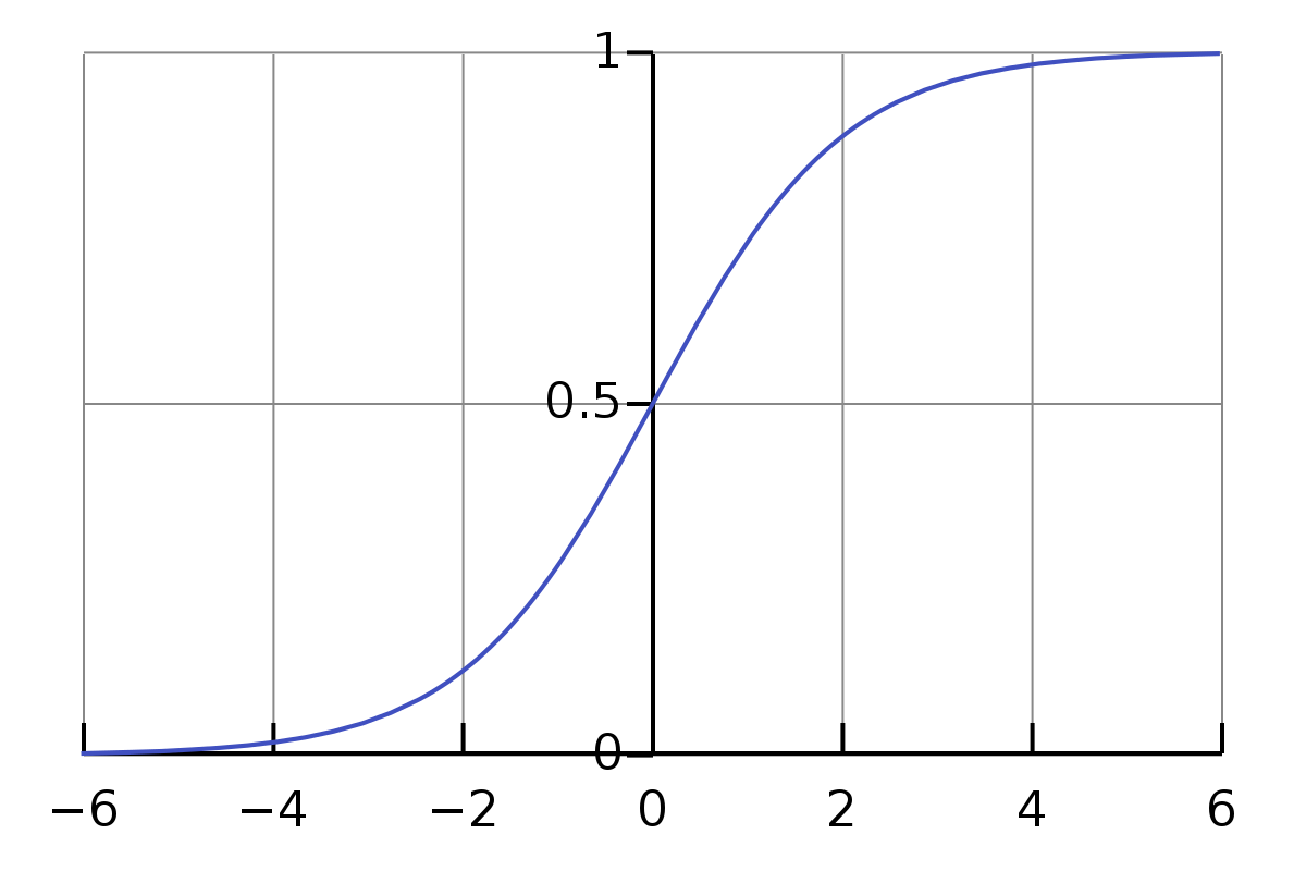
1. What was the formula for the sigmoid function?
\sigma=\frac{1}{1+e^{-z}}
2. Why do we need the sigmoid function? How does it look like?
Questions
3. Can we use any other type of function?

The sigmoid function is what we call Activation Function
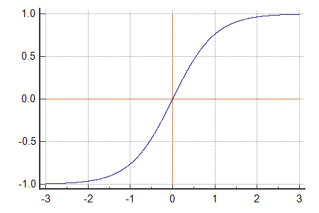
Activation Functions
a = \sigma(z)=\frac{1}{1+e^{-z}}
a = tanh(z)
Activation Functions
a = max(0, z)
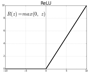
Rectified Linear Unit
(ReLU)
Note: The activation function can vary across the layers
Each of these activation functions has a derivative
[Question: Why do we need to know the derivatives? :) ]
g'(z) = \frac{d}{dz}g(z) = a(1-a)
a = g(z)
Note
\sigma | tanh | ReLU = g
g = \sigma
GIF Time! Too many things going on

Which parameters do we have until now?
Our Parameters
x_1
x_2
x_3
\hat{y}
z^{[1]}_1=w^{[1]T}+b^{[1]}_1
a^{[1]}_1 = \sigma(z^{[1]}_1)
z^{[1]}_2=w^{[1]T}+b^{[1]}_2
a^{[1]}_2 = \sigma(z^{[1]}_2)
z^{[1]}_3=w^{[1]T}+b^{[1]}_3
a^{[1]}_3 = \sigma(z^{[1]}_3)
z^{[2]}_1=w^{[2]T}+b^{[2]}_1
a^{[2]}_1 = \sigma(z^{[2]}_1)
W^{[1]}
= [w^{[1]}_1, w^{[1]}_2, w^{[1]}_3]
This is a matrix!
Our Parameters
x_1
x_2
x_3
\hat{y}
z^{[1]}_1=w^{[1]T}+b^{[1]}_1
a^{[1]}_1 = \sigma(z^{[1]}_1)
z^{[1]}_2=w^{[1]T}+b^{[1]}_2
a^{[1]}_2 = \sigma(z^{[1]}_2)
z^{[1]}_3=w^{[1]T}+b^{[1]}_3
a^{[1]}_3 = \sigma(z^{[1]}_3)
z^{[2]}_1=w^{[2]T}+b^{[2]}_1
a^{[2]}_1 = \sigma(z^{[2]}_1)
W^{[1]}
b^{[1]}
= [b^{[1]}_1, b^{[1]}_2, b^{[1]}_3]
Is b a vector or a matrix?
A: It is a vector
Our Parameters
x_1
x_2
x_3
\hat{y}
z^{[1]}_1=w^{[1]T}+b^{[1]}_1
a^{[1]}_1 = \sigma(z^{[1]}_1)
z^{[1]}_2=w^{[1]T}+b^{[1]}_2
a^{[1]}_2 = \sigma(z^{[1]}_2)
z^{[1]}_3=w^{[1]T}+b^{[1]}_3
a^{[1]}_3 = \sigma(z^{[1]}_3)
z^{[2]}_1=w^{[2]T}+b^{[2]}_1
a^{[2]}_1 = \sigma(z^{[2]}_1)
W^{[1]}
b^{[1]}
W^{[2]}
b^{[2]}
J(W^{[1]}, b^{[1]}, W^{[2]}, b^{[2]})
= \frac{1}{m} \sum
Our Parameters
x_1
x_2
x_3
\hat{y}
z^{[1]}_1=w^{[1]T}+b^{[1]}_1
a^{[1]}_1 = \sigma(z^{[1]}_1)
z^{[1]}_2=w^{[1]T}+b^{[1]}_2
a^{[1]}_2 = \sigma(z^{[1]}_2)
z^{[1]}_3=w^{[1]T}+b^{[1]}_3
a^{[1]}_3 = \sigma(z^{[1]}_3)
z^{[2]}_1=w^{[2]T}+b^{[2]}_1
a^{[2]}_1 = \sigma(z^{[2]}_1)
W^{[1]}
b^{[1]}
W^{[2]}
b^{[2]}
J(W^{[1]}, b^{[1]}, W^{[2]}, b^{[2]})
= \frac{1}{m} \sum^{m}_{i=1}
Our Parameters
x_1
x_2
x_3
\hat{y}
z^{[1]}_1=w^{[1]T}+b^{[1]}_1
a^{[1]}_1 = \sigma(z^{[1]}_1)
z^{[1]}_2=w^{[1]T}+b^{[1]}_2
a^{[1]}_2 = \sigma(z^{[1]}_2)
z^{[1]}_3=w^{[1]T}+b^{[1]}_3
a^{[1]}_3 = \sigma(z^{[1]}_3)
z^{[2]}_1=w^{[2]T}+b^{[2]}_1
a^{[2]}_1 = \sigma(z^{[2]}_1)
W^{[1]}
b^{[1]}
W^{[2]}
b^{[2]}
J(W^{[1]}, b^{[1]}, W^{[2]}, b^{[2]})
= \frac{1}{m} \sum^{m}_{i=1} L(\hat{y}, y)
a^{[2]}
Now we need to calculate the derivatives - we must go backwards
Note: from now on we shall use the vectorized formulas
Summary: Vecorized Forward propagation
X
W
b
z=W^T+b
\hat{y} = a = \sigma(z)
L(\hat{y}, y) = L(a, y)
Summary: Vecorized Forward propagation
x_1
x_2
x_3
\hat{y}
z^{[1]}_1=w^{[1]T}+b^{[1]}_1
a^{[1]}_1 = \sigma(z^{[1]}_1)
z^{[1]}_2=w^{[1]T}+b^{[1]}_2
a^{[1]}_2 = \sigma(z^{[1]}_2)
z^{[1]}_3=w^{[1]T}+b^{[1]}_3
a^{[1]}_3 = \sigma(z^{[1]}_3)
z^{[2]}_1=w^{[2]T}+b^{[2]}_1
a^{[2]}_1 = \sigma(z^{[2]}_1)
Z^{[1]} = W^{[1]}X + b^{[1]}
A^{[1]} = g^{[1]}[Z^{[1]}]
Z^{[2]} = W^{[2]}A^{[1]} + b^{[2]}
A^{[2]} = g^{[2]}[Z^{[2]}]
Summary: Vecorized backward propagation
x
w
b
z=w^T+b
\hat{y} = a = \sigma(z)
L(\hat{y}, y) = L(a, y)
Summary: Vecorized backward propagation
x_1
x_2
x_3
\hat{y}
z^{[1]}_1=w^{[1]T}+b^{[1]}_1
a^{[1]}_1 = \sigma(z^{[1]}_1)
z^{[1]}_2=w^{[1]T}+b^{[1]}_2
a^{[1]}_2 = \sigma(z^{[1]}_2)
z^{[1]}_3=w^{[1]T}+b^{[1]}_3
a^{[1]}_3 = \sigma(z^{[1]}_3)
z^{[2]}_1=w^{[2]T}+b^{[2]}_1
a^{[2]}_1 = \sigma(z^{[2]}_1)
dZ^{[2]} = A^{[2]} - Y
dW^{[2]} = \frac{1}{m}dZ^{[2]}A^{[1]T}
db^{[2]} \approx \frac{1}{m}dZ^{[2]}
dZ^{[1]} = W^{[2]T}dZ^{[2]}*g^{[1]}(Z{[1]})
dW^{[1]} = \frac{1}{m}dZ^{[1]}X^{T}
db^{[1]} \approx \frac{1}{m}dZ^{[1]}

Last tip: randomly initialize the values of W and b.
<3
Canada
\alpha ?
Will the gradient always work?
What's the best activation function?
How many hidden layers should I have?
Agenda
- Why is deep learning so popular now?
- Introduction to Machine Learning
- Introduction to Neural Networks
- Deep Neural Networks
- Training and measuring the performance of the N.N.
- Regularization
- Creating Deep Learning Projects
- CNNs and RNNs
- (OPTIONAL): Tensorflow intro
Source: https://medium.freecodecamp.org/want-to-know-how-deep-learning-works-heres-a-quick-guide-for-everyone-1aedeca88076
x_1
x_2
x_3
x_4
x_5
\hat{y}
6 Layers; L=6
n^{[l]}
=number of units in a layer L
n^{[1]}=6
n^{[2]}=7
n^{[3]}=7
n^{[4]}=6
n^{[5]}=5
n^{[6]}=1
n^{[0]}=5
What should we compute in each of these layers L?
1. Forward step: Z and A
General idea
Z^{[l]} = W^{[l]}A^{[l-1]} + b^{[l]}
A^{[l]} = g^{[l]}(Z^{[l]})
Input:
A^{[l-1]}
Output:
A^{[l]}
Z works like a cache
2. Backpropagation: derivatives
General idea
Input:
dA^{[l]}
Output:
dA^{[l-1]}, dW{[l]}
db{[l]}
Basic building block
In a layer l,

Forward
Backprop
A^{[l-1]}
A^{[l]}
W^{[l]}
b^{[l]}
cache Z^{[l]}
dA^{[l]}
dA^{[l-1]}
dZ^{[l]}
dW^{[l]} , db^{[l]}

<3
Canada
My predictions are awful. HELP
Agenda
- Why is deep learning so popular now?
- Introduction to Machine Learning
- Introduction to Neural Networks
- Deep Neural Networks
- Training and measuring the performance of the N.N.
- Regularization
- Creating Deep Learning Projects
- CNNs and RNNs
- (OPTIONAL): Tensorflow intro
When should I stop training?
Select a fraction of your data set to check which model performs best.
Once you find the best model, make a final test (unbiased estimate)
Data
Training set
C.V. = Cross Validation set (select the best model)
C.V.
T = Test set (unbiased estimate)
T
Problem
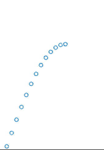
h(x) = \theta_0 + \theta_1x
Does it look good?
Underfitting
h(x) = \theta_0 + \theta_1x
The predicted output is not even fitting the training data!
Problem
h(x) = \theta_0 + \theta_1x + \theta_2x^2
+ \theta_3x^3 + \theta_4x^4
Does it look good?
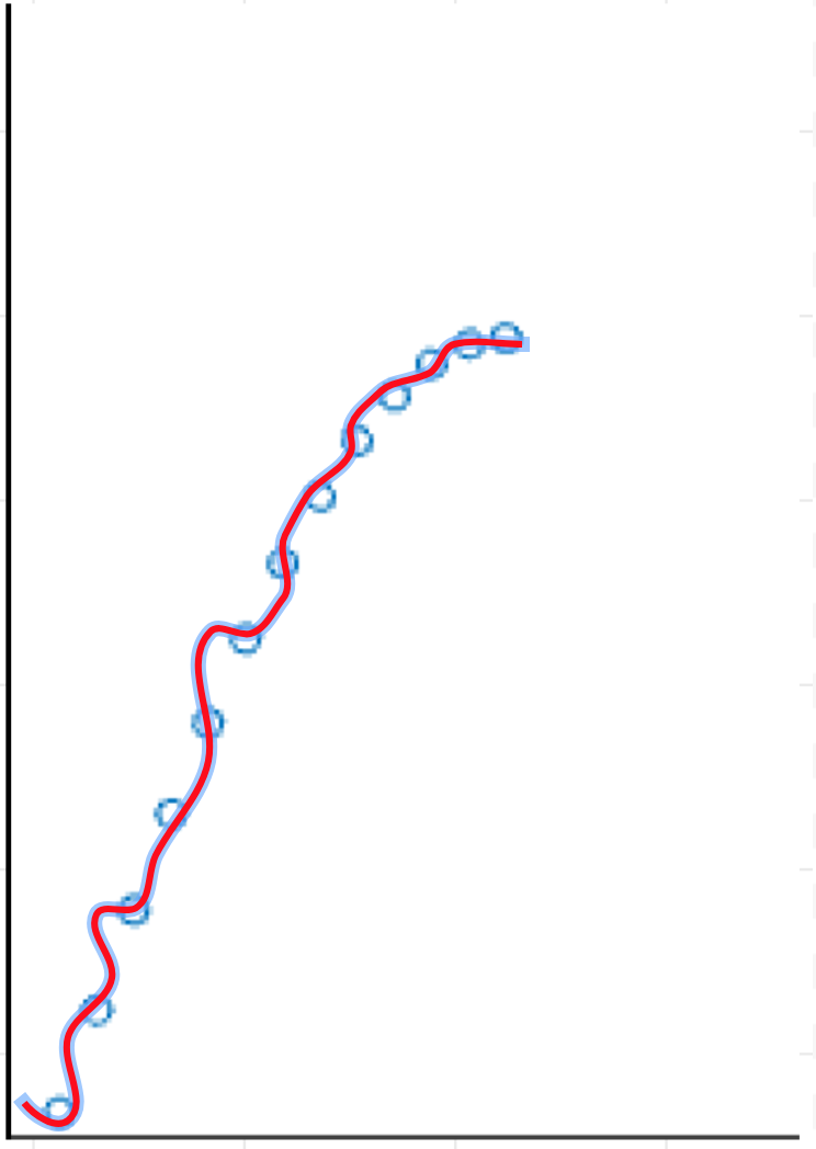
Overfitting
h(x) = \theta_0 + \theta_1x + \theta_2x^2
+ \theta_3x^3 + \theta_4x^4
The model fits everything
[Over, Under]fitting are problems related to the capacity
Capacity: Ability to fit a wide variety of functions
Overfitting
Underfitting
[Over, Under]fitting are problems related to the capacity
Capacity: Ability to fit a wide variety of functions
High variance
High Bias
How can we properly identify bias and variance problems?
A: check the error rates of the training and C.V. sets
| Training set error | 1% |
|---|---|
| C.V. Error | 11% |
High variance problem
| Training set error | 15% |
|---|---|
| C.V. Error | 16% |
High bias problem
(not even fitting the training set properly!)
| Training set error | 15% |
|---|---|
| C.V. Error | 36% |
High bias problem AND high variance problem
How can we control the capacity?
Are you fitting the data of the training set?
No
High bias
Bigger network (more hidden layers and units)
Train more
Different N.N. architecture
Yes
Is your C.V. error low?
No
High variance
More data
Regularization
Different N.N. architecture
Yes
DONE!
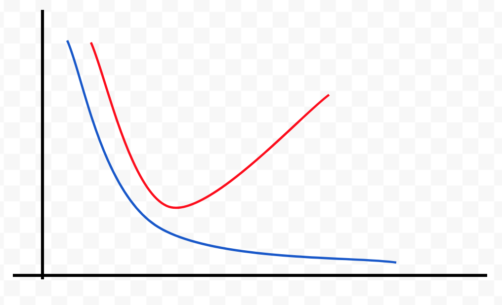
Error
Capacity
J(θ) test error
J(θ) train error
Error
Capacity
J(θ) cv error
J(θ) train error
Bias problem (underfitting)
J(θ) train error is high
J(θ) train ≈ J(θ) cv
J(θ) train error is low
J(θ) cv >> J(θ) train
Variance problem (overfitting)
Error
Capacity
J(θ) test error
J(θ) train error
Stop here!

Let's talk about overfitting
Why does it happen?
You end up having a very complex N.N., with the elements of the matrix W being too large.
x_1
x_2
x_3
\hat{y}
w: HIIIIIIIIIIIIIIIIII
w: HELOOO
w: WOAHHH
w: !!111!!!
W's with a strong presence in every layer can cause overfitting. How can we solve that?
x_1
x_2
x_3
\hat{y}
w: HIIIIIIIIIIIIIIIIII
w: HELOOO
w: WOAHHH
w: !!111!!!
\lambda
SHH
HHHHHH
Who is
\lambda ?
Agenda
- Why is deep learning so popular now?
- Introduction to Machine Learning
- Introduction to Neural Networks
- Deep Neural Networks
- Training and measuring the performance of the N.N.
- Regularization
- Creating Deep Learning Projects
- CNNs and RNNs
- (OPTIONAL): Tensorflow intro
Regularization paramter
\lambda
It penalizes the W matrix for being too large.
\lambda
In terms of mathematics, how does it happen?
\lambda
W^{[l]}
\lambda
W^{[l]}
Norm
Norm
||W^{[l]}||^2
L2-Norm (Euclidean)
||W^{[l]}||
L1-Norm
{||W^{[l]}||}{^2}{_F}
Forbenius Norm
Final combo (L2-norm)
J(W^{[1]}, b^{[1]}, ..., W^{[l]}, b^{[l]}) =
\frac{1}{m} \sum^{m}_{i=1} L(\hat{y}, y)
+\frac{\lambda}{2m}
||W^{[l]}||^2
||W^{[l]}||^2 = \sum^{N_x}_{j=1} wj^2 = w^tw
<3
Canada
Are there other ways to perform regularization, without calculating a norm?
More slides here (Part II):
https://slides.com/hannelitavante-hannelita/deep-learning-unifei-ii#/
Deep Learning UNIFEI
By Hanneli Tavante (hannelita)


