Probabilistic Programming for Cosmology with JAX

Hugo SIMON-ONFROY,
PhD student supervised by
Arnaud DE MATTIA and François LANUSSE
CoPhy, 2024/11/19
The universe recipe (so far)
$$\frac{H}{H_0} = \sqrt{\Omega_r + \Omega_b + \Omega_c+ \Omega_\kappa + \Omega_\Lambda}$$
instantaneous expansion rate
energy content
Cosmological principle + Einstein equation
+ Inflation
\(\delta_L \sim \mathcal G(0, \mathcal P)\)
\(\sigma_8:= \sigma[\delta_L * \boldsymbol 1_{r \leq 8}]\)
initial field
primordial power spectrum
std. of fluctuations smoothed at \(8 \text{ Mpc}/h\)
\(\Omega := \{ \Omega_c, \Omega_b, \Omega_\Lambda, H_0, \sigma_8, n_s,...\}\)

Linear matter spectrum
Structure growth
Cosmological modeling and inference
\(\Omega\)
\(\delta_L\)
\(\delta_g\)
inference
Please define model
Model: an observation generator, link between latent and observed variables
\(F\)
\(C\)
\(D\)
\(E\)
\(A\)
\(B\)
\(G\)
Frequentist:
fixed but unknown parameters
Bayesian:
random because unknown
\(A\)
\(B\)
\(C\)
\(F\)
\(D\)
\(E\)
\(G\)
Represented as a DAG which expresses a joint probability factorization, i.e. conditional dependencies between variables
latent param
latent variable
observed variable
Definitions
evidence/prior predictive: $$\boldsymbol{p}(y) := \int \boldsymbol{p}(y \mid x) \boldsymbol{p}(x)d x$$
posterior predictive: $$\boldsymbol{p}(y_1 \mid y_0) := \int \boldsymbol{p}(y_1 \mid x) \boldsymbol{p}(x \mid y_0)d x$$
\(Y\)
\(X\)
Bayes thm
\(\sim\)
\(\underbrace{\boldsymbol{p}(x \mid y)}_{\text{posterior}}\underbrace{\boldsymbol{p}(y)}_{\text{evidence}} = \underbrace{\boldsymbol{p}(y \mid x)}_{\text{likelihood}} \,\underbrace{\boldsymbol{p}(x)}_{\text{prior}}\)
\(Y\)
\(X\)
Marginalization:
\(Y\)
\(X\)
\(Z\)
\(Z\)
\(X\)
\(Y\)
\(X\)
Conditioning/Bayes inversion:
\(Y\)
\(X\)
Definitions
evidence/prior predictive: $$\boldsymbol{p}(y) := \int \boldsymbol{p}(y \mid x) \boldsymbol{p}(x)d x$$
posterior predictive: $$\boldsymbol{p}(y_1 \mid y_0) := \int \boldsymbol{p}(y_1 \mid x) \boldsymbol{p}(x \mid y_0)d x$$
\(Y\)
\(X\)
Conditioning/Bayes inversion:
\(X\)
\(Z\)
Marginalization:
\(Y\)
\(X\)
Bayes thm
\(\sim\)
\(\underbrace{\boldsymbol{p}(x \mid y)}_{\text{posterior}}\underbrace{\boldsymbol{p}(y)}_{\text{evidence}} = \underbrace{\boldsymbol{p}(y \mid x)}_{\text{likelihood}} \,\underbrace{\boldsymbol{p}(x)}_{\text{prior}}\)
\(Y\)
\(X\)

\(s\)
\(\Omega\)
Cosmology is (sometimes) hard
Typical cosmological analyses
Field-level inference
Summary stat inference
\(\delta_g\)
\(b\)
\(\Omega\)
\(\delta_g\)
\(b\)
\(\Omega\)
\(\delta_L\)
\(b\)
\(\Omega\)
\(s\)
\(\delta_g\)
\(b\)
\(\Omega\)
\(\delta_L\)
\(\delta_g\)
\(\delta_L\)
\(s\)
marginalize
invert
marginalize
invert
\(b\)
\(\Omega\)
\(s\)
\(\delta_g\)
\(b\)
\(\Omega\)
\(\delta_L\)
\(\delta_L\)
Probabilistic Programming: Wish List
\(\begin{cases}x,y,z \text{ samples}\\\boldsymbol{p}(x,y,z)\\\Phi= -\log \boldsymbol{p}\\\nabla\Phi,\nabla^2 \Phi,\dots\end{cases}\)
1. Modeling
e.g. in JAX with \(\texttt{NumPyro}\), \(\texttt{JaxCosmo}\), \(\texttt{JaxPM}\), \(\texttt{DISCO-EB}\)...
2. DAG compilation
PPLs e.g. \(\texttt{NumPyro}\), \(\texttt{Stan}\), \(\texttt{PyMC}\)...
3. Inference
e.g. MCMC or VI with \(\texttt{NumPyro}\), \(\texttt{Stan}\), \(\texttt{PyMC}\), \(\texttt{emcee}\)...
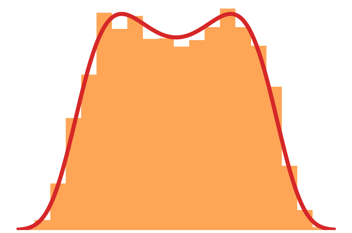
4. Extract and viz
e.g. KDE with \(\texttt{GetDist}\), \(\texttt{GMM-MI}\), \(\texttt{mean()}\), \(\texttt{std()}\)...
Physics job
Stats job
Stats job
auto!
\(X\)
\(Z\)
\(Y\)
\(X\)
\(Z\)
1
2
3
4

Benchmarking preconditionning
$$\underbrace{\mathcal C\mathcal N (\delta_{\text{obs}} \mid b_K \delta_L, \frac{1}{\bar n}I)}_{\text{likelihood}}\;\underbrace{\mathcal C \mathcal N(\delta_L \mid 0, P_L)}_{\text{prior}} = \underbrace{\mathcal C\mathcal N(\delta_L \mid \mu, \sigma^2 I)}_{\text{posterior}}\; \underbrace{\mathcal C \mathcal N(\delta_0 \mid 0, \frac{1}{\bar n}I+b_K^2 P_L)}_{\text{evidence}}$$
$$\text{with } \begin{cases}b_K &:= (1+ b_1 + f \mu_k^2)D \\ \sigma&:= (\bar n b_K^2 + P_L^{-1})^{-1/2} \\ \mu &:= \sigma^2\bar n b_K \delta_{\text{obs}}\\ \end{cases}$$
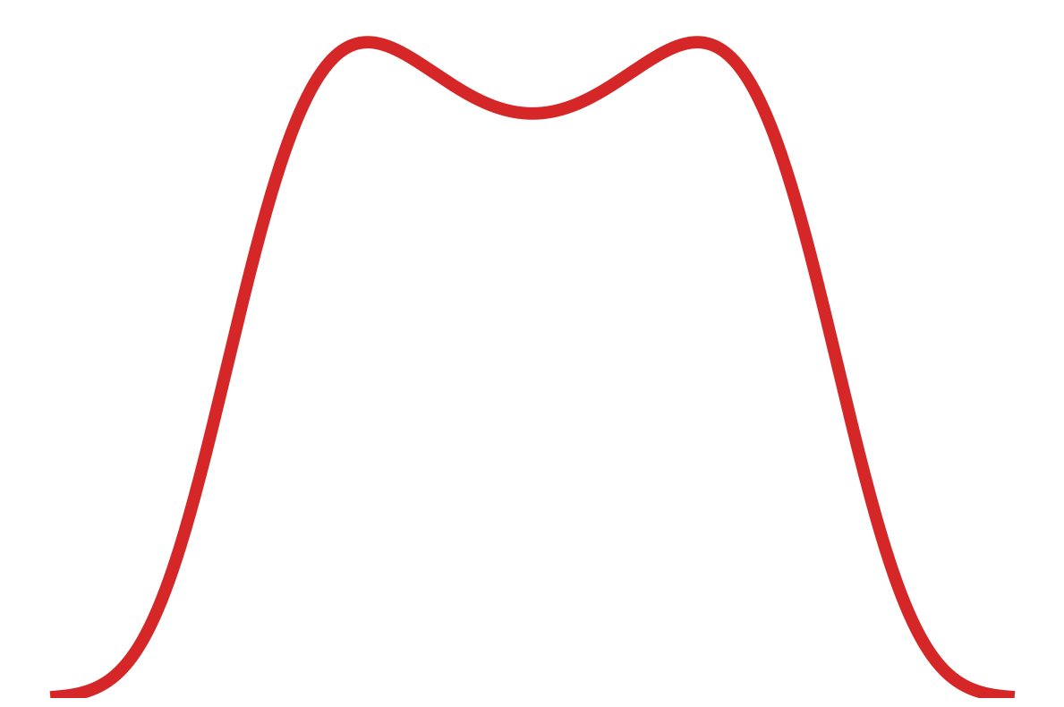
- To optimize sampling efficiency, the posterior should be an isotropic Gaussian. So if it is not, we should reparametrize the model such that it is.
- To precondition efficiently, we assume a Kaiser model:
linear growth + linear Eulerian bias + flat sky RSD + Gaussian noise
- We can compute posterior analytically:
😊
😔


Benchmarking samplers

unadjusted and Micro-Canonical Langevin Monte Carlo (MCLMC) scales better than s.o.t.a. NUTS/HMC for higher dimensional sampling problems
Finalizing scaling tests: what happens at higher resolution? N-body evolution?
Some useful programming tools
-
NumPyro
- Probabilistic Programming Language (PPL)
- Powered by JAX
- Integrated samplers
-
JAX
-
GPU acceleration
- Just-In-Time (JIT) compilation acceleration
- Automatic vectorization/parallelization
- Automatic differentiation
-
GPU acceleration
JAX reminder
-
GPU accelerate
- JIT compile
- Vectorize/Parallelize
- Auto-diff
import jax.numpy as np
# then enjoy
function = jax.jit(function)
# function is so fast now!gradient = jax.grad(function)
# too bad if you love chain ruling by handvfunction = jax.vmap(function)
pfunction = jax.pmap(function)
# for-loops are for-loosersProbabilistic Modeling and Compilation
def simulate(seed):
    rng = np.random.RandomState(seed)
    x = rng.randn()
    y = rng.randn() + x**2
    return x, y
from scipy.stats import norm
log_prior = lambda x: norm.logpdf(x, 0, 1)
log_lik = lambda x, y: norm.logpdf(y, x**2, 1)
log_joint= lambda x, y: log_lik(y, x) + log_prior(x)grad_log_prior = lambda x: x**2
grad_log_lik = lambda x, y: stack([2 * x * (y - x**2), (y - x**2)])
grad_log_joint = lambda x, y: grad_log_lik(y, x) + stack([grad_log_prior(x), zeros_like(y)])
# Hessian left as an exercise...To fully define a probabilistic model, we need
- its simulator
- its associated joint log prob
- possibly its gradients, Hessian... (useful for inference)
We should only care about the simulator!
\(Y\)
\(X\)
$$\begin{cases}X \sim \mathcal N(0,1)\\Y\mid X \sim \mathcal N(X^2, 1)\end{cases}$$
my model on paper
my model on code
What if we modify to fit variances? non-Gaussian dist? Recompute everything? :'(
Modeling with Numpyro


y_sample = seed(model, 42)()
log_joint = lambda x, y: log_density(model,(),{},{'x':x, 'y':y})[0]
obs_model = condition(model, y_sample)
logp_fn = lambda x: log_density(obs_model,(),{},{'x':x})[0]def model():
x = sample('x', dist.Normal(0, 1))
y = sample('y', dist.Normal(x**2, 1))
return yfrom jax import jit, vmap, grad
force_vfn = jit(vmap(grad(logp_fn)))- Define model as simulator... and that's it
- Simulate, get log prob
- +JAX machinery
- Condition model
- And more!
So NumPyro in practice?
def model():
    x = sample('x', dist.Normal(0, 1))
    y = sample('y', dist.Normal(x**2, 1))
    return y
render_model(model, render_distributions=True)
y_sample = dict(y=seed(model, 42)())
obs_model = condition(model, x_sample)
logp_fn = lambda x: log_density(obs_model,(),{},{'x':x})[0]from jax import jit, vmap, grad
force_vfn = jit(vmap(grad(logp_fn)))kernel = infer.NUTS(obs_model)
mcmc = infer.MCMC(kernel, num_warmup, num_samples)
mcmc.run(jr.key(43))
samples = mcmc.get_samples()- Probabilistic Programming
- JAX machinery
- Integrated samplers
Why care about differentiable model?
-
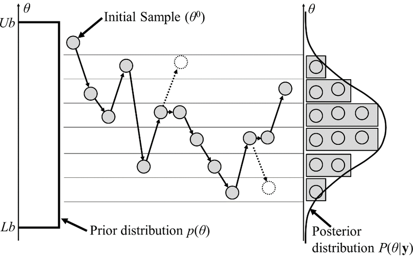
Classical MCMCs
-
agnostic random moves
+ MH acceptance step
= blinded natural selection
- small moves yield correlated samples
-
agnostic random moves
- SOTA MCMCs rely on the gradient of the model log-prob, to drive dynamic towards highest density regions

gradient descent
posterior mode
Brownian
exploding Gaussian
Langevin
posterior
+
=
Hamiltonian Monte Carlo (HMC)
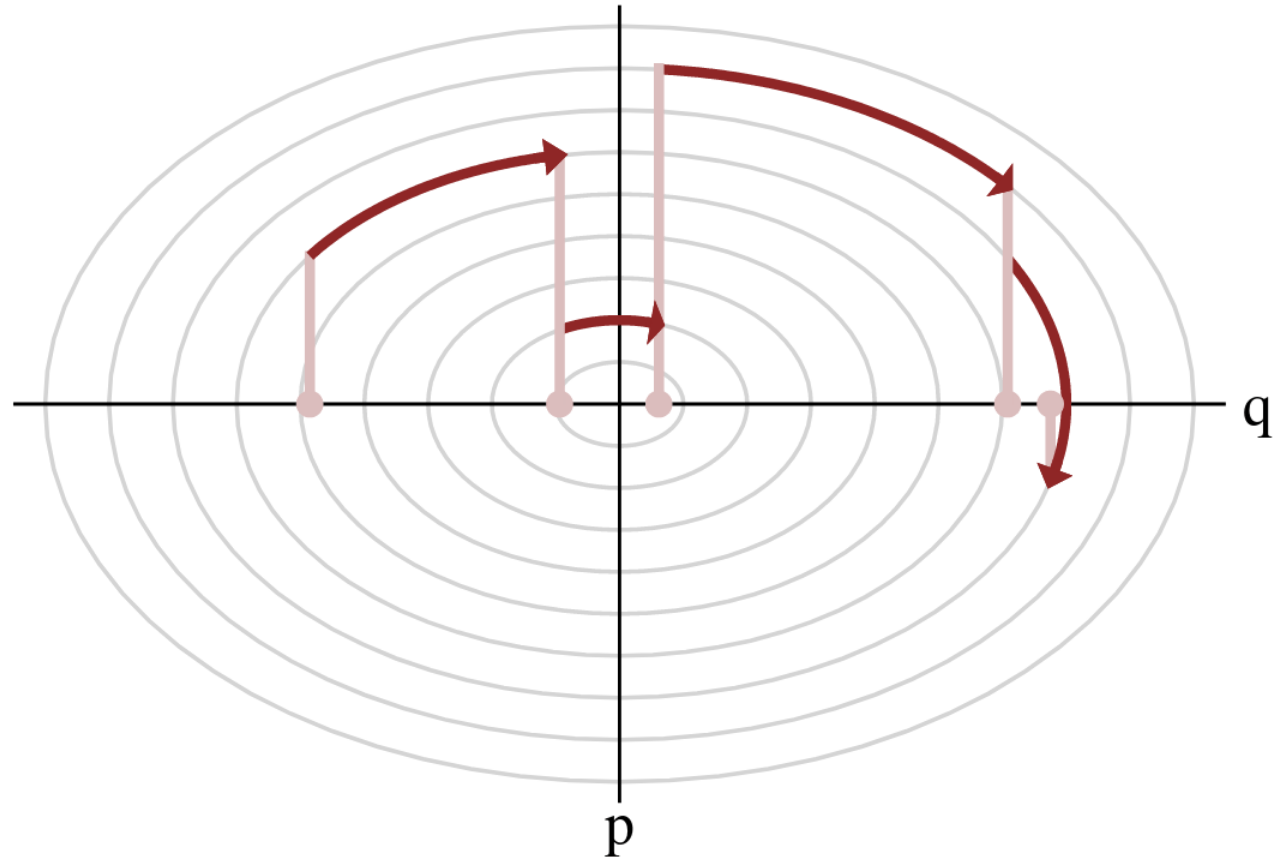
- To travel farther, add inertia.
- sample particle at position \(q\) now have momentum \(p\) and mass matrix \(M\)
- target \(\boldsymbol{p}(q)\) becomes \(\boldsymbol{p}(q , p) := e^{-\mathcal H(q,p)}\), with Hamiltonian $$\mathcal H(q,p) := -\log \boldsymbol{p}(q) + \frac 1 2 p^\top M^{-1} p$$
- at each step, resample momentum \(p \sim \mathcal N(0,M)\)
- let \((q,p)\) follow the Hamiltonian dynamic during time length \(L\), then arrival becomes new MH proposal.

Variations around HMC
-
No U-Turn Sampler (NUTS)
- trajectory length \(L\) auto-tuned
- samples drawn along trajectory
- NUTSGibbs i.e. alternating sampling over parameter subsets.
Why care about differentiable model?
Variations around HMC
-
No U-Turn Sampler (NUTS)
- trajectory length auto-tuned
- samples drawn along trajectory
- NUTSGibbs i.e. alternating sampling over parameter subsets
-
Model gradient drives sample particles towards high density regions
-
Hamiltonian Monte Carlo (HMC):
to travel farther, add inertia
- Yields less correlated chains
3) Hamiltonian dynamic
1) mass \(M\) particle at \(q\)
2) random kick \(p\)
2) random kick \(p\)
1) mass \(M\) particle at \(q\)
3) Hamiltonian dynamic
Why care about differentiable model?
-
Model gradient drives sample particles towards high density regions
-
Hamiltonian Monte Carlo (HMC):
to travel farther, add inertia
- Yields less correlated chains
3) Hamiltonian dynamic
1) mass \(M\) particle at \(q\)
2) random kick \(p\)
2) random kick \(p\)
1) mass \(M\) particle at \(q\)
3) Hamiltonian dynamic

Inference with NumPyro
def model():
    x = sample('x', dist.Normal(0, 1))
    y = sample('y', dist.Normal(x**2, 1))
    return y

render_model(model, render_distributions=True)

y_sample = dict(y=seed(model, 42)())
obs_model = condition(model, x_sample)
logp_fn = lambda x: log_density(obs_model,(),{},{'x':x})[0]
from jax import jit, vmap, grad
force_vfn = jit(vmap(grad(logp_fn)))kernel = infer.NUTS(obs_model)
mcmc = infer.MCMC(kernel, num_warmup, num_samples)
mcmc.run(jr.key(43))
samples = mcmc.get_samples()- Probabilistic Model
- +JAX machinery
- = gradient-based MCMC
How to N-body-differentiate?


\((q, p)\)
\(\delta(x)\)
\(\delta(k)\)
paint*
read*
fft*
ifft*
fft*
*: differentiable, e.g. with , see JaxPM
apply forces
to move particles
solve Vlasov-Poisson
to compute forces

- Prior on
- Cosmology \(\Omega\)
- Initial field \(\delta_L\)
- Dark matter-galaxy connection (Lagrangian galaxy biases) \(b\)
- Initialize matter particles
- LSS formation (LPT+PM)
- Populate matter field with galaxies
- Galaxy peculiar velocities (RSD)
- Observational noise
Let's build a cosmological model


- Fast and differentiable model thx to JaxPM
- still, \(\simeq 1024^3\) parameters is huge!
- Some proposed methods by Lavaux+2018, Bayer+2023
Which sampling methods can scale to high dimensions?
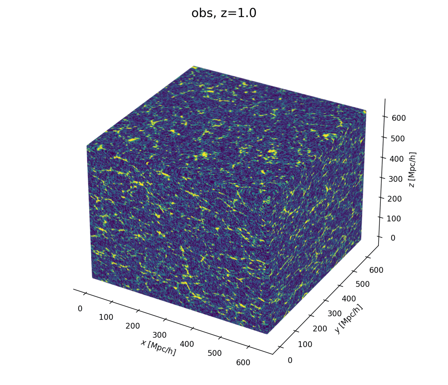
- At large scales, matter density field almost Gaussian so power spectrum is almost lossless compression
- At smaller scales however, matter density field non-Gaussian
Gaussianity and beyond
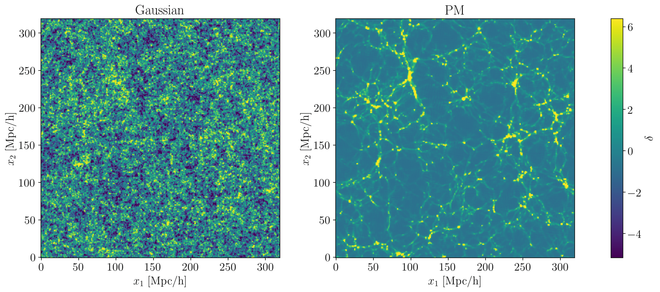
2 fields, 1 power spectrum: Gaussian or N-body?
-
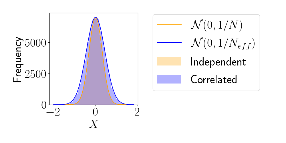
Effective Sample Size (ESS)
- number of i.i.d. samples that yield same statistical power.
- For sample sequence of size \(N\) and autocorrelation \(\rho\) $$N_\textrm{eff} = \frac{N}{1+2 \sum_{t=1}^{+\infty}\rho_t}$$so aim for as less correlated sample as possible.
- Main limiting computational factor is model evaluation (e.g. N-body), so characterize MCMC efficiency by \(N_\text{eval} / N_\text{eff}\)
How to compare samplers?
2024CoPhy
By hsimonfroy


