


Ishanu Chattopadhyay PRO
ML Data Science Biomedicine Social Science Faculty
Ishanu Chattopadhyay
University of Chicago
CCTS 40500 / CCTS 20500 / BIOS 29208
Winter 2023
Lecture 3
Contact
ishanu@uchicago.edu
900 E57 ST
KCBD 10152
Room: BSLC 313
Monday 9.30 - 12.20 AM
Resources
https://github.com/zeroknowledgediscovery/course_notes
RCC Midway
RCC Midway
ssh -X username@midway2.rcc.uchicago.edu
screen
sinteractive --exclusive --time=08:00:00
login
get a compute node within screen
module load python
a=`/sbin/ip route get 8.8.8.8 | awk '{print $NF;exit}'`
jupyter-notebook --no-browser --ip="$a"
start jupyter notebook without browser
Access the notebook from local machine
/project2/ishanu/run_jupyter.sh
simplify
RCC Midway
# open terminal

screen
sinteractive --exclusive --time=08:00:00
login
get a compute node within screen
module load python
a=`/sbin/ip route get 8.8.8.8 | awk '{print $NF;exit}'`
jupyter-notebook --no-browser --ip="$a"
start jupyter notebook without browser
Access the notebook from local machine
/project2/ishanu/run_jupyter.sh
simplify
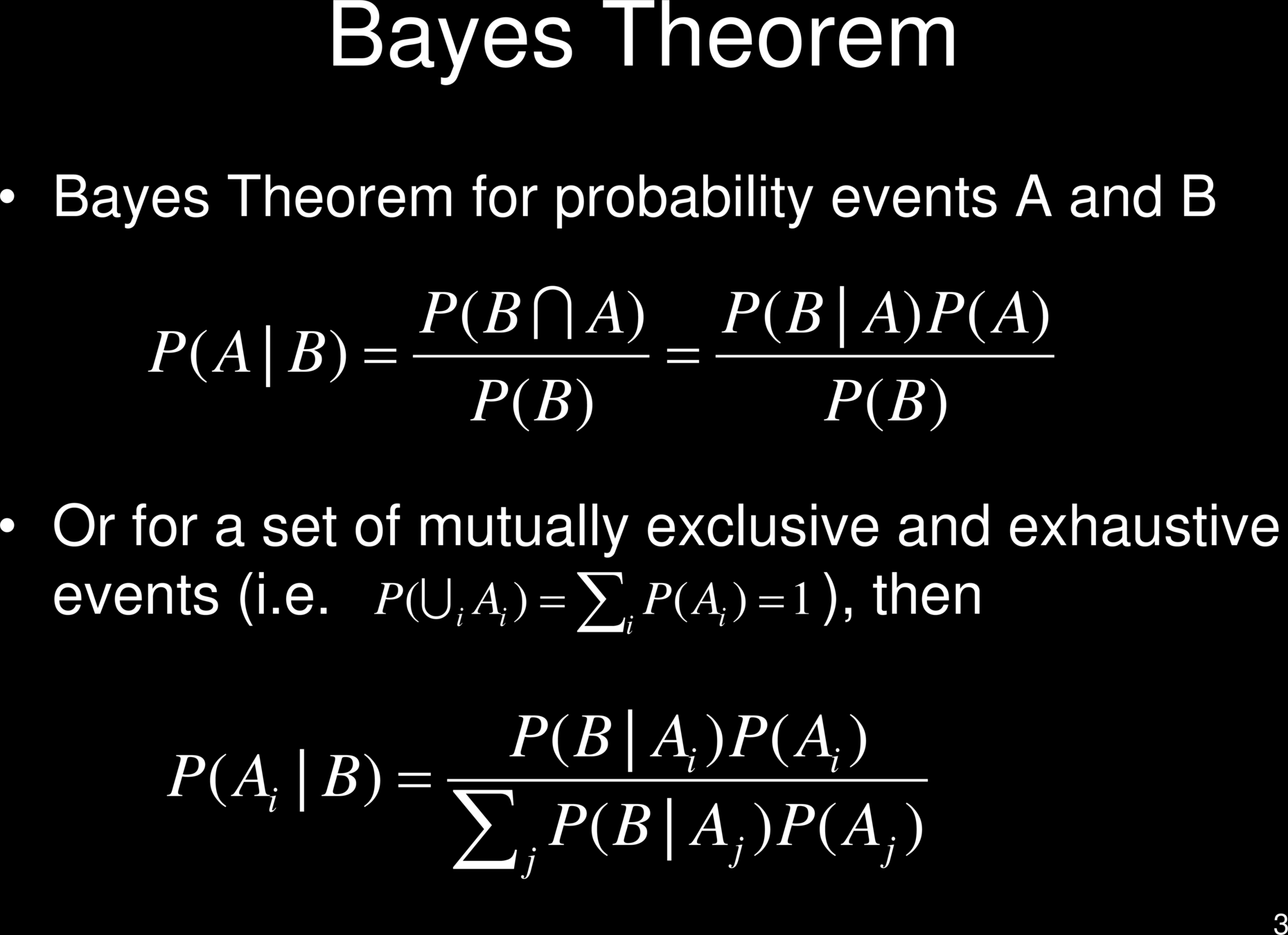
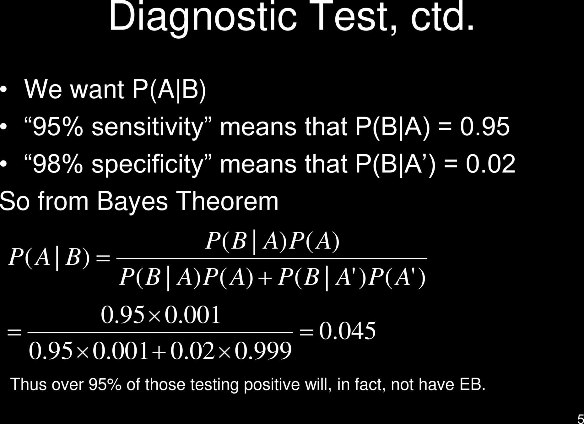
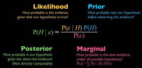
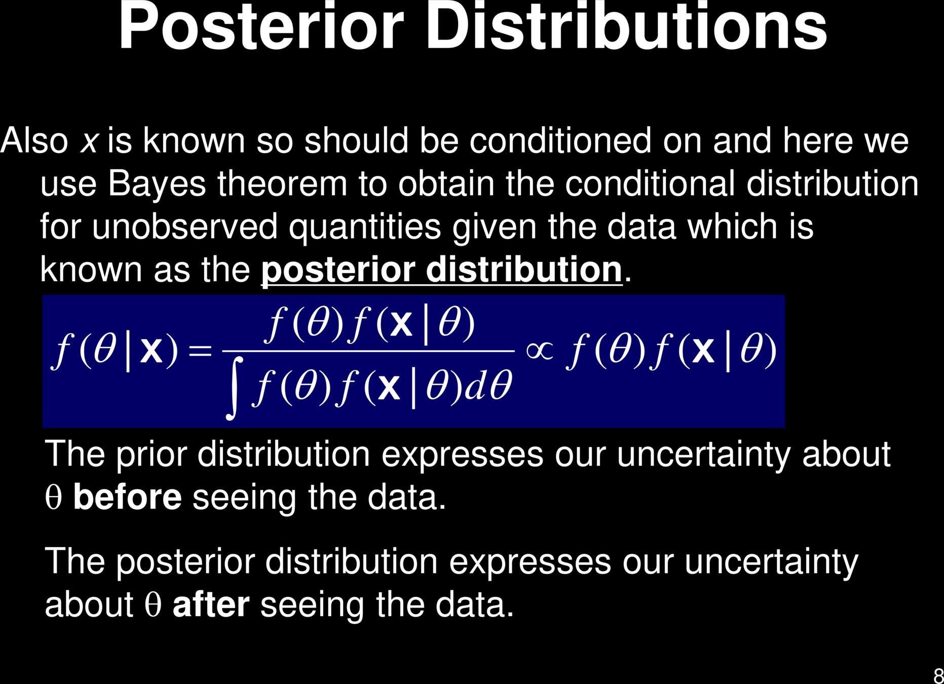
Bayesian Statistics
Bayes' Error
Decision Trees
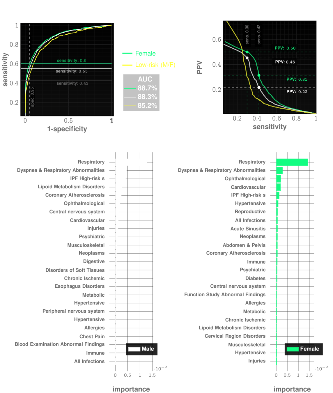
prevalence is intrinsic property of the disease
Idiopathic Pulmonary Fibrosis
prevalence: ~0.5%
The decision threshold is upto us to decide
Impacts sensitivity & specificity
| Cost | Positive | Negative |
|---|---|---|
| Test Positive | $0 | $x |
| Test Negative | $y | $0 |
Cost Optimization to choose operating point
Criminal Justice: $$C(f_n) = 0 $$
Healthcare: $$C(f_p) = 0 $$
naive dichotomy
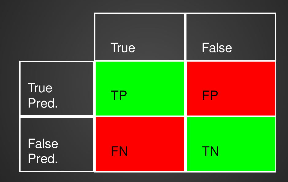
Classification & Decision Theory
Classification & Decision Theory
Classification & Decision Theory
Classification & Decision Theory
Classification & Decision Theory
Mathematical definition of classifier:
Risk of a classifier:
Classification & Decision Theory
Bayes Risk
Risk of a classifier:
Mathematical definition of classifier:
search over all possible classifiers
Classification & Decision Theory
Bayes Risk
A classifier achieving the Bayes risk is a Bayes Optimal Classifier
Bayesian Decision Theory
Minimizing the 0, 1-loss is equivalent to minimizing the overall misclassification rate. 0, 1-loss is an example of a symmetric loss function: all errors are penalized equally. In certain applications, asymmetric loss functions are more appropriate.
Recall cost of false negatives vs that of false positives
The expected 0, 1-loss is precisely the probability of making a mistake
Defining Bayes Optimal Classifier in terms of the Loss function
Bayesian Decision Theory
Bayes Optimal Classifier
The above derivation is of course for only 0-1 Loss
But this is true in general
Bayes Optimal Classifier: Example
Assume we want to classify fish based on length
Bayes Optimal Classifier: Example
Assume we want to classify fish based on length
Why doesn't this solve all problems in ML?
Bayes Risk
Bayes Risk
Bayes Risk
Bayes Optimal Classifier
What happens if the loss function is more general?
HW
extra credit
if x == y
  class = 0
else
  class = 1
N1: is x == 1 ? (yes -> N2, no -> N3)
N2: is y == 1 ? (yes -> class=0, no -> class=1)
N3: is y == 1 ? (yes -> class=1, no -> class=0)XOR
HW
We will look at Q-nets later that optimally solve this problem
Key Problem: Overfitting
Formal Description of Overfitting
How Does Overfitting Look Like In Practice?
How Does Overfitting Look Like In Practice?
Are More Features Always Better? NO
Advantages of decision trees are:
The disadvantages of decision trees include:
Decision-tree learners can create over-complex trees that do not generalise the data well. This is called overfitting. Mechanisms such as pruning, setting the minimum number of samples required at a leaf node or setting the maximum depth of the tree are necessary to avoid this problem.
Decision trees can be unstable because small variations in the data might result in a completely different tree being generated. This problem is mitigated by using decision trees within an ensemble.
Predictions of decision trees are neither smooth nor continuous, but piecewise constant approximations. Therefore, they are not good at extrapolation.
The problem of learning an optimal decision tree is known to be NP-complete under several aspects of optimality and even for simple concepts. Consequently, practical decision-tree learning algorithms are based on heuristic algorithms such as the greedy algorithm where locally optimal decisions are made at each node. Such algorithms cannot guarantee to return the globally optimal decision tree. This can be mitigated by training multiple trees in an ensemble learner, where the features and samples are randomly sampled with replacement.
There are concepts that are hard to learn because decision trees do not express them easily, such as XOR, parity or multiplexer problems.
Decision tree learners create biased trees if some classes dominate. It is therefore recommended to balance the dataset prior to fitting with the decision tree.
How do we make decision trees better?
Reduce "bias"
Reduce "variance"
Cannot reduce "irreducible error"
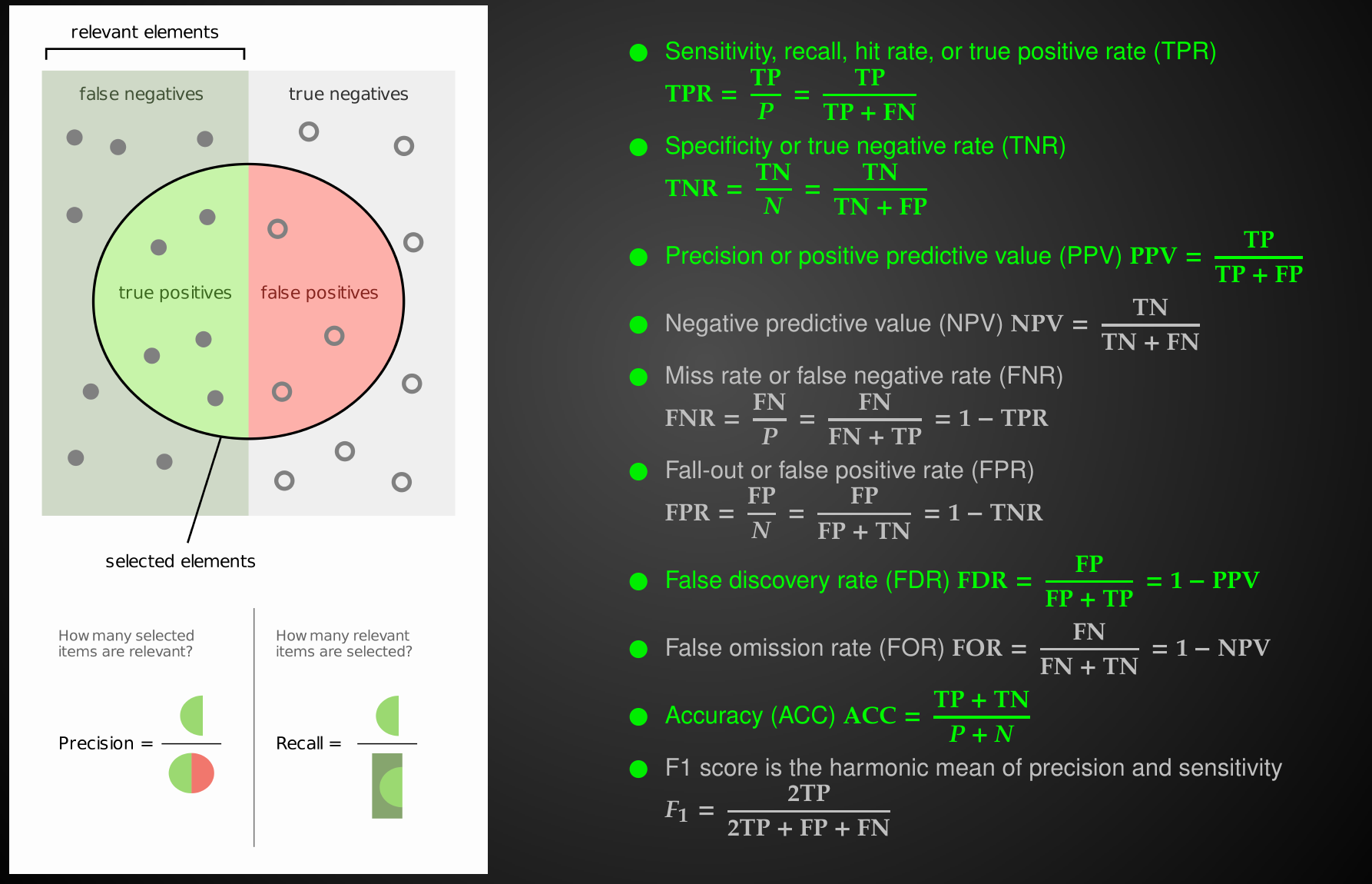
Note: performance metrics relate to the sample population, not to individual samples
THE TABULAR DATA FORMAT
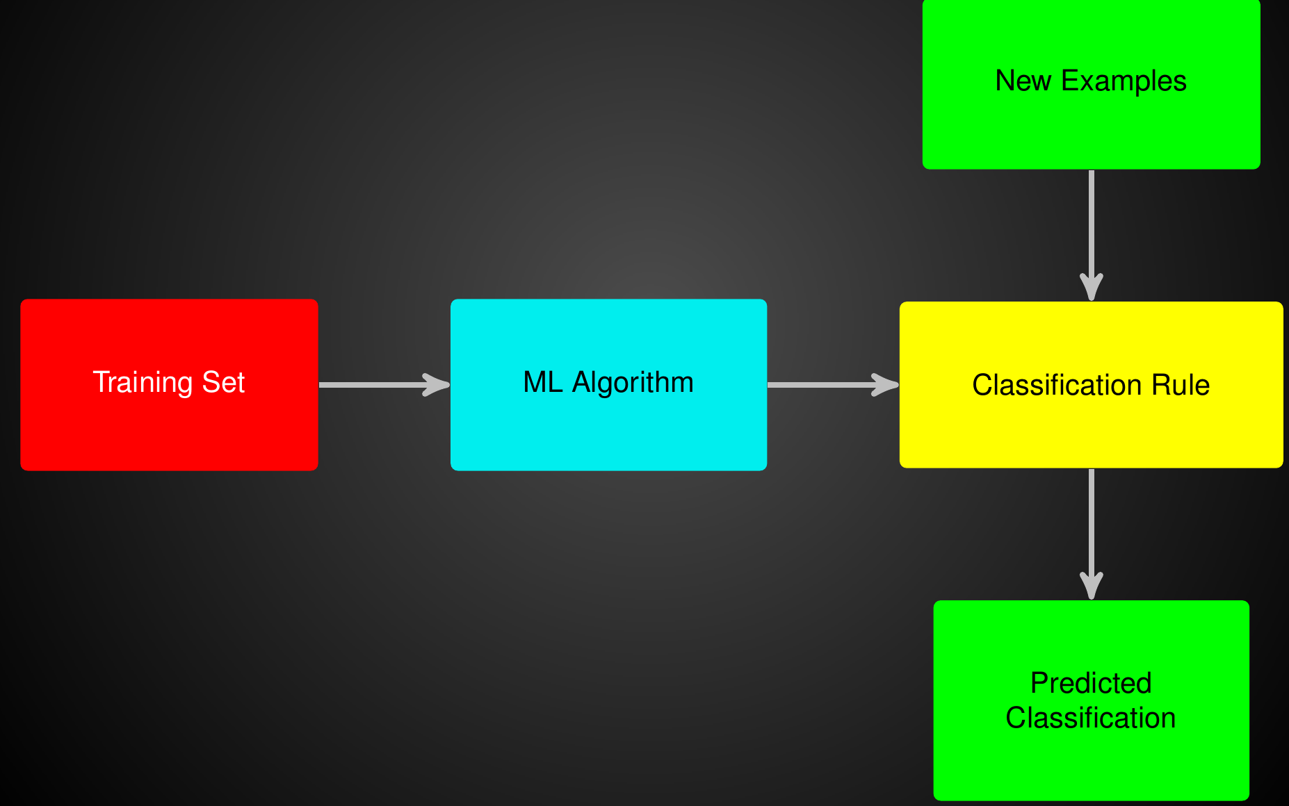
Summing Up The ML Problem
Naive Bayes Assumption
Expected Test Error:
bias
variance
irreducible error
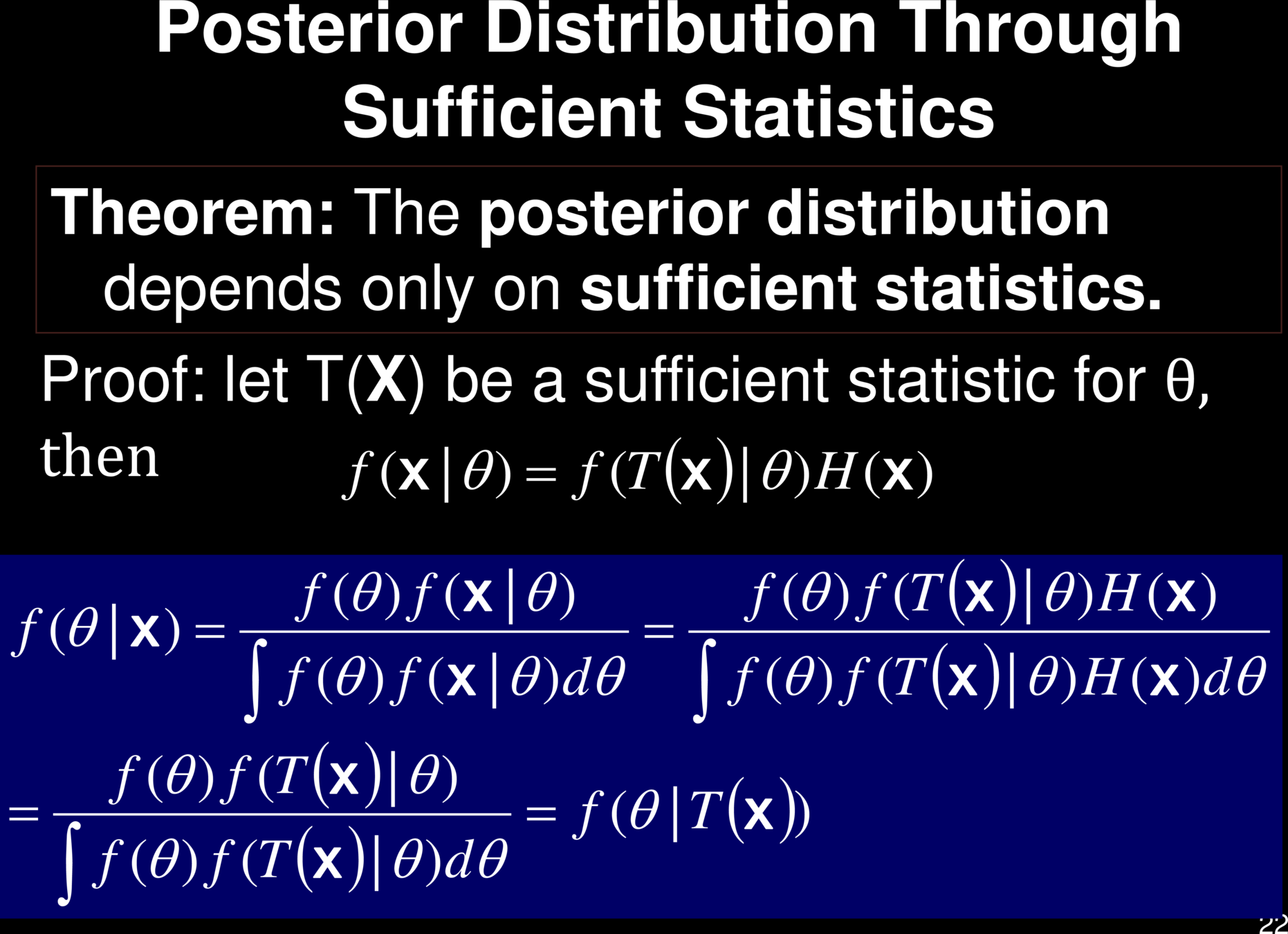
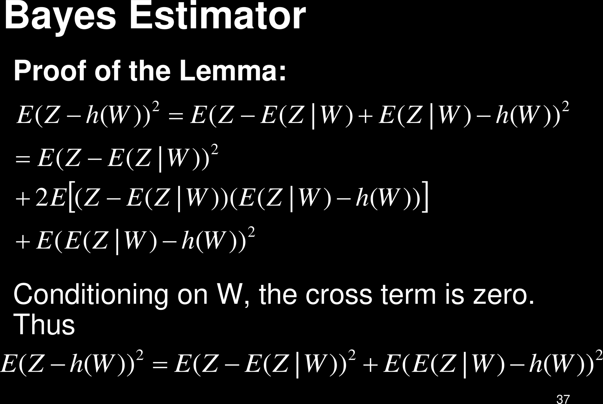
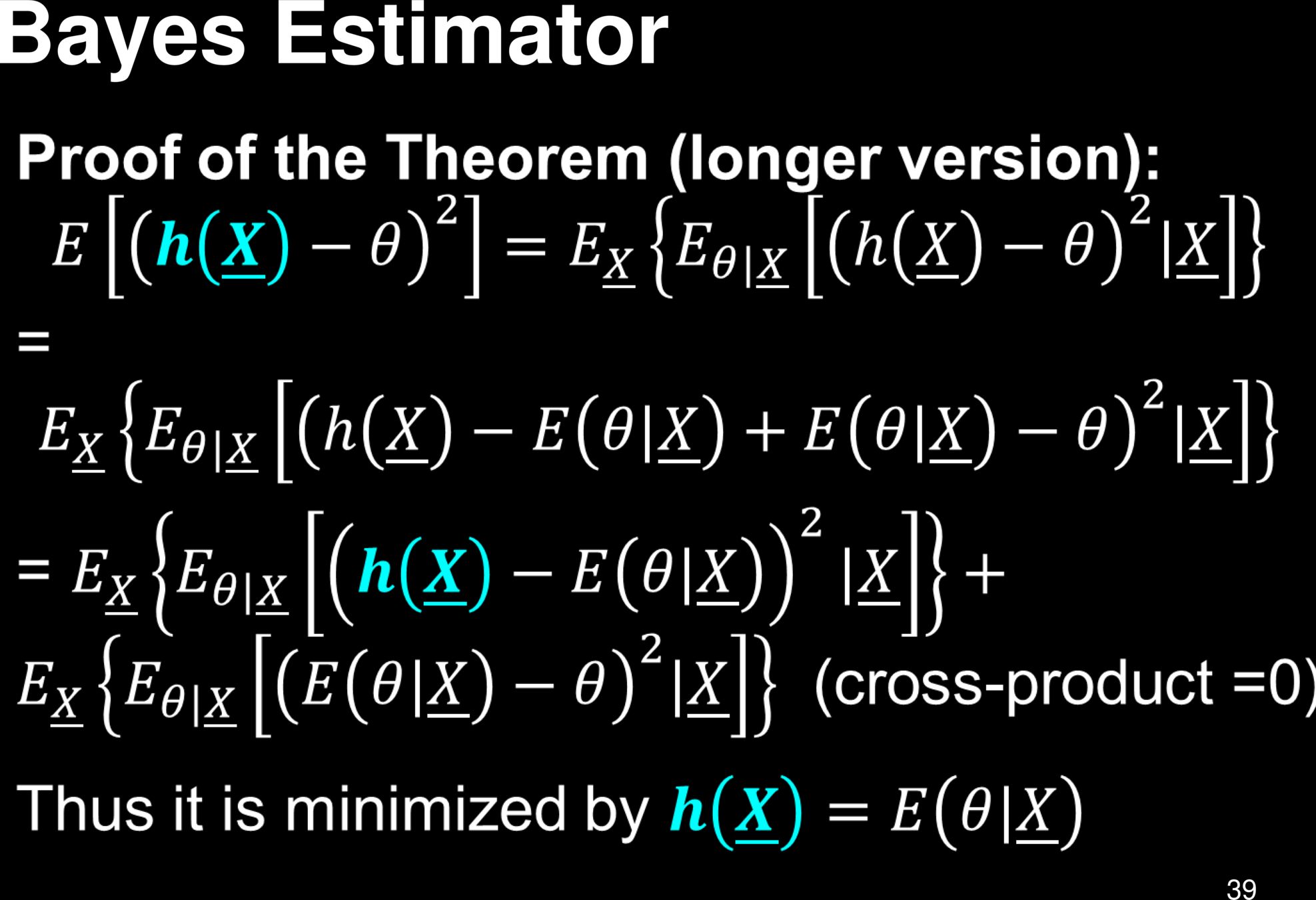
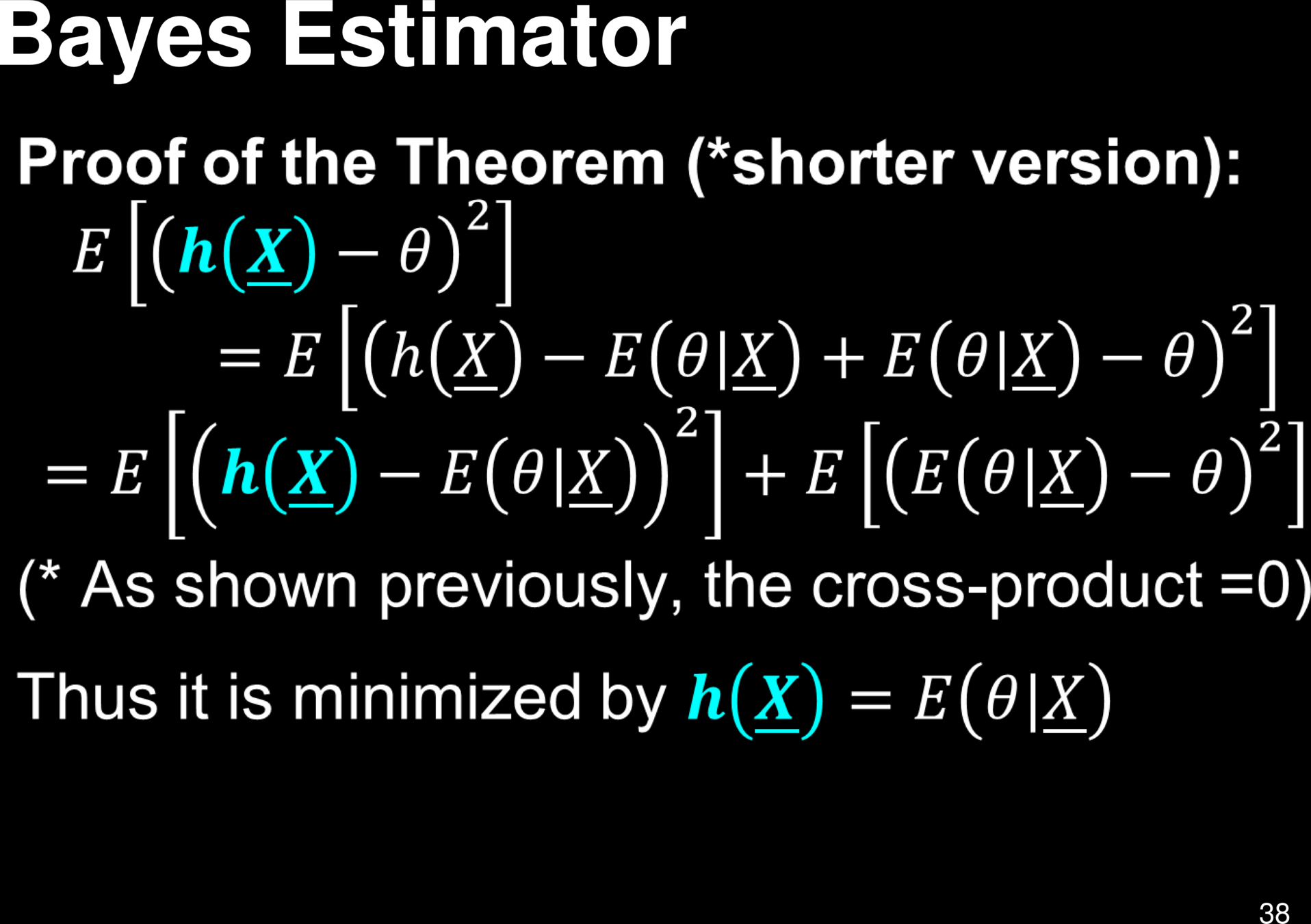
Show Proof
from sklearn.model_selection import train_test_split
from sklearn import metrics
from sklearn.tree import DecisionTreeClassifier
from sklearn.ensemble import BaggingClassifier

clf_ = DecisionTreeClassifier(max_depth=4, class_weight='balanced')
clf = BaggingClassifier(base_estimator=clf_,n_estimators=10,oob_score=True)
X_train, X_test, y_train, y_test = train_test_split(X, y, test_size=0.2)
clf.fit(X_train,y_train)
clf.predict(X_test,y_test)Average over the feature importance of base models
Median might be better
import numpy as np
from sklearn.ensemble import BaggingClassifier
from sklearn.tree import DecisionTreeClassifier
from sklearn.datasets import load_iris

X, y = load_iris(return_X_y=True)
clf = BaggingClassifier(DecisionTreeClassifier())
clf.fit(X, y)

feature_importances = np.mean([
    tree.feature_importances_ for tree in clf.estimators_
], axis=0)
Average over the feature importance of base models
Median might be better
Instead of one "rule", it is a distribution over rules, or a linear combination of rules
HW. Prove this
Proof here:
What happens when there is one strongly predicting feature?
How do we avoid this?
We can penalize the number of times a feature is used at a certain depth
We can penalize the number of times a feature can be used
We will only allow some features chosen by some meta analysis
No! Same Bias
No! Same Bias
No! Same Bias
from sklearn.ensemble import RandomForestClassifier
clf = RandomForestClassifier(max_depth=None, class_weight='balanced',n_estimators=300)
y_pred = clf.fit(X_train, y_train).predict(X_test)
By Ishanu Chattopadhyay
Machine Learning for Biomedicine


