Day 33:
The Vandermonde Matrix and
fitting functions to data
Definition. Given a collection of numbers
\[x_{1},x_{2},x_{3},\ldots,x_{m}\]
and a number \(n\in\N\), the \(m\times n\) matrix
\[\begin{bmatrix}1 & x_{1} & x_{1}^{2} & \cdots & x_{1}^{n-1}\\[1ex] 1 & x_{2} & x_{2}^{2} & \cdots & x_{2}^{n-1}\\[1ex] 1 & x_{3} & x_{3}^{2} & \cdots & x_{3}^{n-1}\\ \vdots & \vdots & \vdots & & \vdots \\ 1 & x_{m} & x_{m}^{2} & \cdots & x_{m}^{n-1}\\\end{bmatrix} \]
is called a Vandermonde matrix.
Theorem. Given a collection of distinct numbers
\[x_{1},x_{2},x_{3},\ldots,x_{m}\]
and a number \(n\leq m\), the \(m\times n\) matrix
\[V = \begin{bmatrix}1 & x_{1} & x_{1}^{2} & \cdots & x_{1}^{n-1}\\[1ex] 1 & x_{2} & x_{2}^{2} & \cdots & x_{2}^{n-1}\\[1ex] 1 & x_{3} & x_{3}^{2} & \cdots & x_{3}^{n-1}\\ \vdots & \vdots & \vdots & & \vdots \\ 1 & x_{m} & x_{m}^{2} & \cdots & x_{m}^{n-1}\\\end{bmatrix} \]
has a trivial nullspace, that is \(N(V)=\{0\}\).
Proof. Suppose there is a nonzero vector \[x = \begin{bmatrix} a_{0} & a_{1} & a_{2} & \cdots & a_{n-1}\end{bmatrix}^{\top}\in N(V).\] This means that \(Vx=0\), that is, for each \(i=1,2,\ldots m\) we have
\[a_{0}+a_{1}x_{i}+a_{2}x_{i}^{2}+a_{3}x_{i}^{3}+\cdots+a_{n-1}x_{i}^{n-1}=0.\]
Proof continued. Define the polynomial
\[f(x) = a_{0}+a_{1}x+a_{2}x^{2}+a_{3}x^{3}+\cdots+a_{n-1}x^{n-1},\]
then we see that \(f\) has \(m\) distinct roots \(x_{1},x_{2},\ldots,x_{m}\). Hence, we can factor \(f(x)\) as follows
\[f(x) = (x-x_{1})(x-x_{2})(x-x_{3})\cdots (x-x_{m})g(x)\]
where \(g(x)\) is some polynomial. From this we see that the degree of \(f(x)\) is at least \(m\), that is, \(n-1\geq m\). This contradicts the assumption that \(n\leq m\). Hence, our assumption at the beginning of the proof must be false, that is, there is no nonzero vector in \(N(V)\). \(\Box\)
Corollary. If \((x_{1},y_{1}),(x_{2},y_{2}),\ldots,(x_{n},y_{n})\) are points in \(\R^{2}\) with distinct first coordinates, then there is a unique degree \(n-1\) polynomial \(p(x)\) such that \[p(x_{i}) = y_{i}\quad\text{for }i=1,2,\ldots,n.\]
Proof. By the previous theorem, the \(n\times n\) matrix
\[V = \begin{bmatrix}1 & x_{1} & x_{1}^{2} & \cdots & x_{1}^{n-1}\\[1ex] 1 & x_{2} & x_{2}^{2} & \cdots & x_{2}^{n-1}\\ \vdots & \vdots & \vdots & & \vdots \\ 1 & x_{n} & x_{n}^{2} & \cdots & x_{n}^{n-1}\\\end{bmatrix} \]
has a trivial nullspace, that is \(N(V)=\{0\}\). Since this matrix is square, it must be full rank, that is, the columns of \(V\) are a basis for \(\R^{n}\). Thus, there is a unique vector\[x=\begin{bmatrix} a_{0} & a_{1} & a_{2} & \cdots & a_{n-1}\end{bmatrix}^{\top}\] such that \(Vx=y\), where \[y=\begin{bmatrix} y_{1} & y_{2} & \cdots & y_{n}\end{bmatrix}^{\top}.\]
Thus \(p(x)=a_{0}+a_{1}x+\cdots+a_{n-1}x^{n-1}\) is the desired polynomial. \(\Box\)
Example. Find the unique \(3\)rd degree polynomial \(p(x)\) such that \[\qquad p(1)=2,\quad p(2)=2,\quad p(3)=-1\quad\text{and}\quad p(4)=6.\]
\[A = \left[\begin{array}{cccc} 1 & 1 & 1 & 1\\ 1 & 2 & 4 & 8\\ 1 & 3 & 9 & 27\\ 1 & 4 & 16 & 64\end{array}\right]\quad\text{and}\quad b=\begin{bmatrix}2\\ 2\\ -1\\ 6\end{bmatrix}\]
From the previous theorem the columns of \(A\) span \(\R^{4}\) and hence \(Ax=b\) has a solution. But, \(A\) is invertible, so there is a unique solution
\[x=A^{-1}b = \begin{bmatrix} -14 & \frac{85}{3} & -\frac{29}{2} & \frac{13}{6}\end{bmatrix}^{\top}\]
Hence, the unique polynomial is
\[p(x) = -14 + \frac{85}{3}x - \frac{29}{2}x^2 + \frac{13}{6}x^3.\]
\[A = \left[\begin{array}{cccc} 1 & 0 & 0 & 0\\ 1 & 1 & 1 & 1\\ 1 & 2 & 4 & 8\\ 1 & 3 & 9 & 27\\ 1 & 4 & 16 & 64\end{array}\right]\quad\text{and}\quad b=\begin{bmatrix}-14\\ 2\\ 2\\ -1\\ 6\end{bmatrix}\]
Note that the columns of \(A\) do not span \(\R^{5}\) (since there are only \(4\) of them!) but \(Ax=b\) still has a solution:
\[x=\begin{bmatrix} -14 & \frac{85}{3} & -\frac{29}{2} & \frac{13}{6}\end{bmatrix}^{\top}.\]
Hence, the desired polynomial exists:
\[p(x) = -14 + \frac{85}{3}x - \frac{29}{2}x^2 + \frac{13}{6}x^3.\]
Example. Find a \(3\)rd degree polynomial \(p(x)\) such that \[\qquad p(1)=2,\quad p(2)=2,\quad p(3)=-1\quad\text{and}\quad p(4)=6.\]
\(p(0)=-14,\)
\[A = \left[\begin{array}{cccc} 1 & 0 & 0 & 0\\ 1 & 1 & 1 & 1\\ 1 & 2 & 4 & 8\\ 1 & 3 & 9 & 27\\ 1 & 4 & 16 & 64\end{array}\right]\quad\text{and}\quad b=\begin{bmatrix}-13\\ 2\\ 2\\ -1\\ 6\end{bmatrix}\]
Example. Find a \(3\)rd degree polynomial \(p(x)\) such that \[\qquad p(1)=2,\quad p(2)=2,\quad p(3)=-1\quad\text{and}\quad p(4)=6.\]
\(p(0)=-13,\)
Now, \(Ax=b\) has no solution! So, there is no \(3\)rd degree polynomial \(p(x)\) with all of the desired properties.
\[A = \left[\begin{array}{cccc} 1 & 0 & 0 & 0\\ 1 & 1 & 1 & 1\\ 1 & 2 & 4 & 8\\ 1 & 3 & 9 & 27\\ 1 & 4 & 16 & 64\end{array}\right]\quad\text{and}\quad b=\begin{bmatrix}-14.01\\ 1.98\\ 2.03\\ -0.99\\ 6\end{bmatrix}\]
Example. Find a \(3\)rd degree polynomial \(p(x)\) such \[p(0)=-14.01,\ p(1)=1.98,\ p(2)=2.03,\ p(3)=-0.99,\text{ and } p(4)=6.\]
We still see that \(Ax=b\) has no solution! So, there is no \(3\)rd degree polynomial \(p(x)\) with all of the desired properties.
But, this is only because of "noise" in \(b\). If we find the least squares solution to \(Ax=b\),
\[\hat{x} = A^{+}b = \begin{bmatrix} -14.013 & 28.3225 & -14.4800 & 2.1625\end{bmatrix}^{\top}\]
Then we see that the "closest" \(3\)rd degree polynomial is \[p(x) = -14.013+28.3225x-14.4800x^2+2.1625x^3,\] where \[p(0)=-14.014,\ p(1) = 1.992,\ p(2)=2.012,\ p(3)=-0.978,\ p(4)=5.997\]


What degree to choose?
\[-0.0367+0.2921x-0.6828 x^2+ 0.5434x^3+ 0.3656x^4\]
What degree to choose?
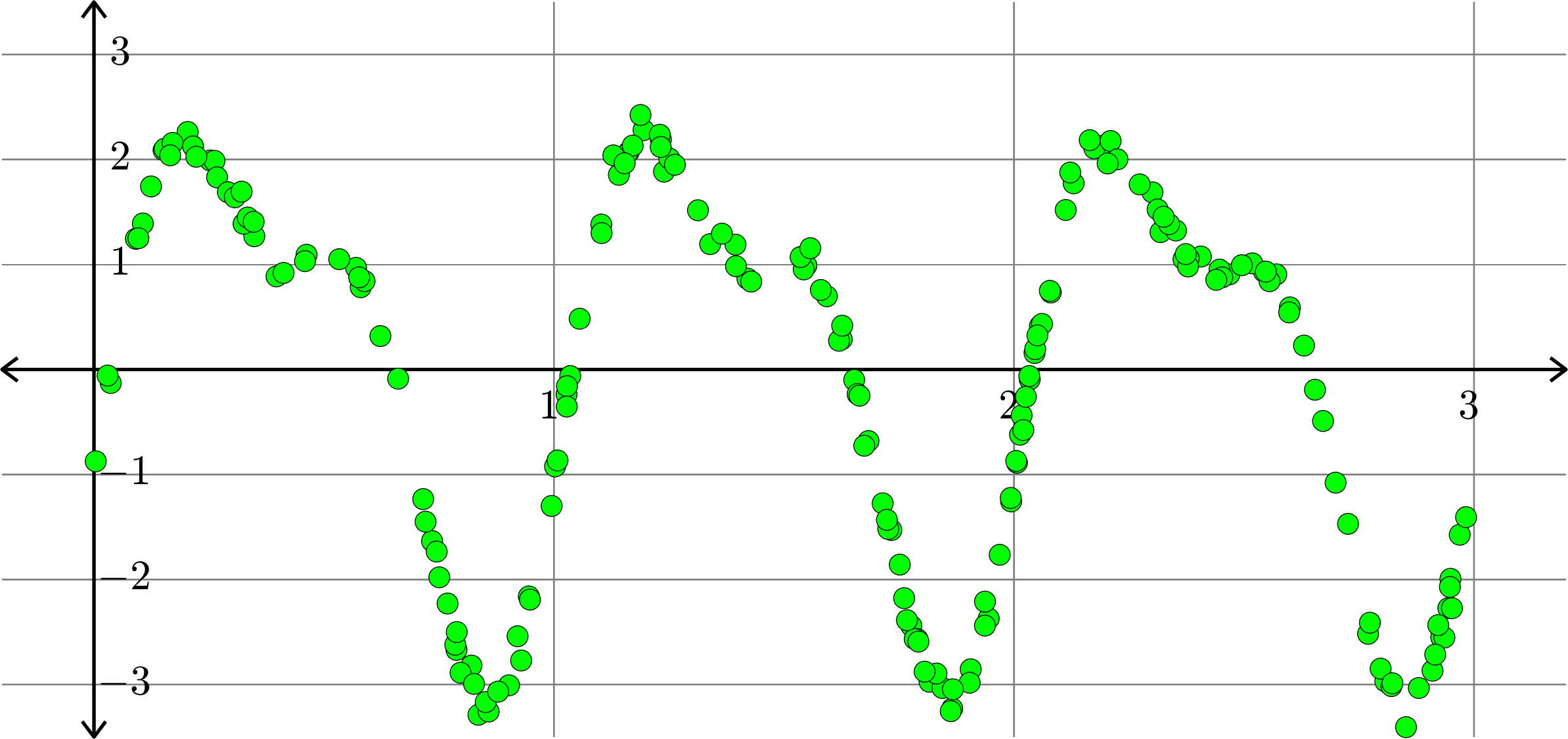


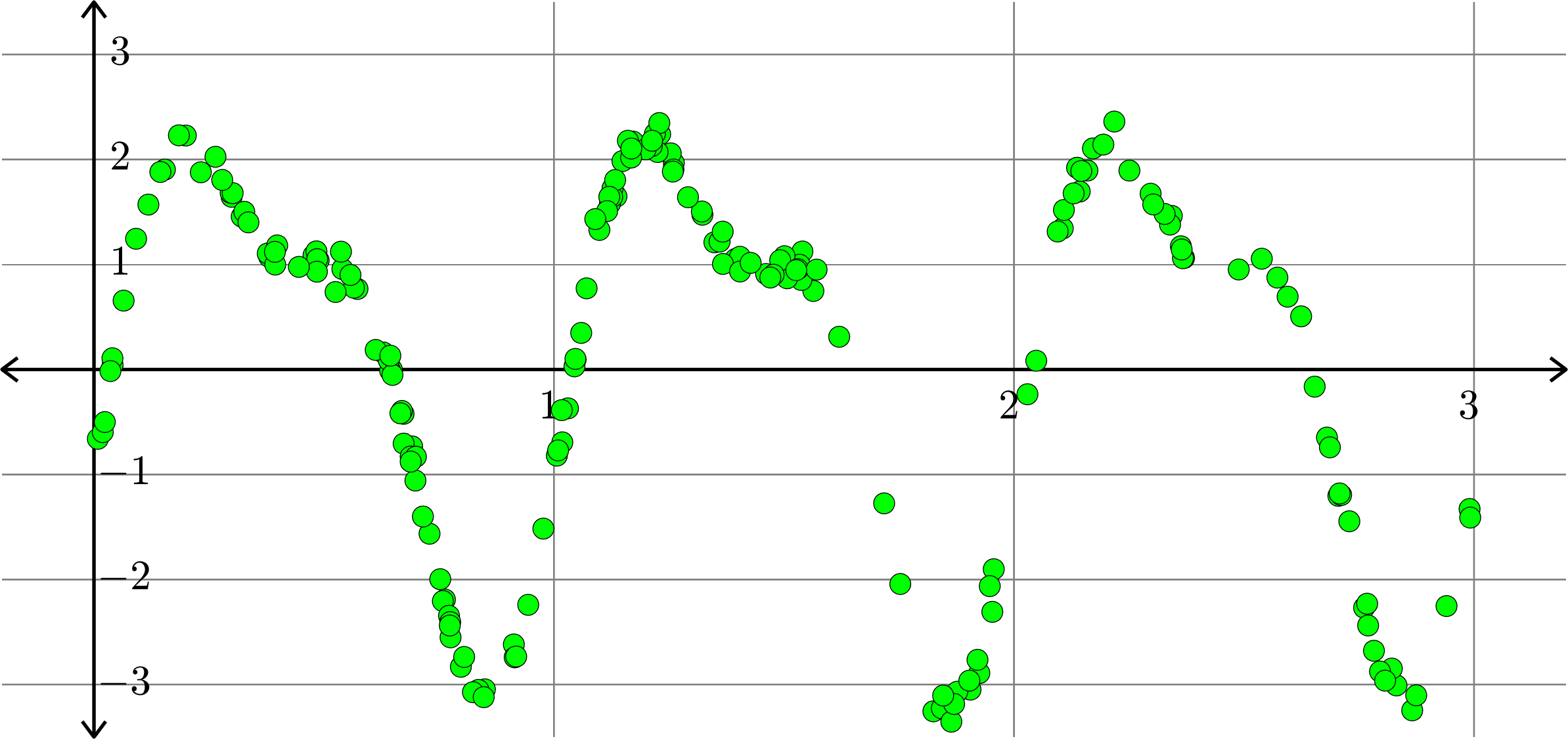
What if polynomials don't fit?
Consider the collection of points in \(\R^{2}\):
\[(x_{1},y_{1}),(x_{2},y_{2}),\ldots,(x_{n},y_{n})\]
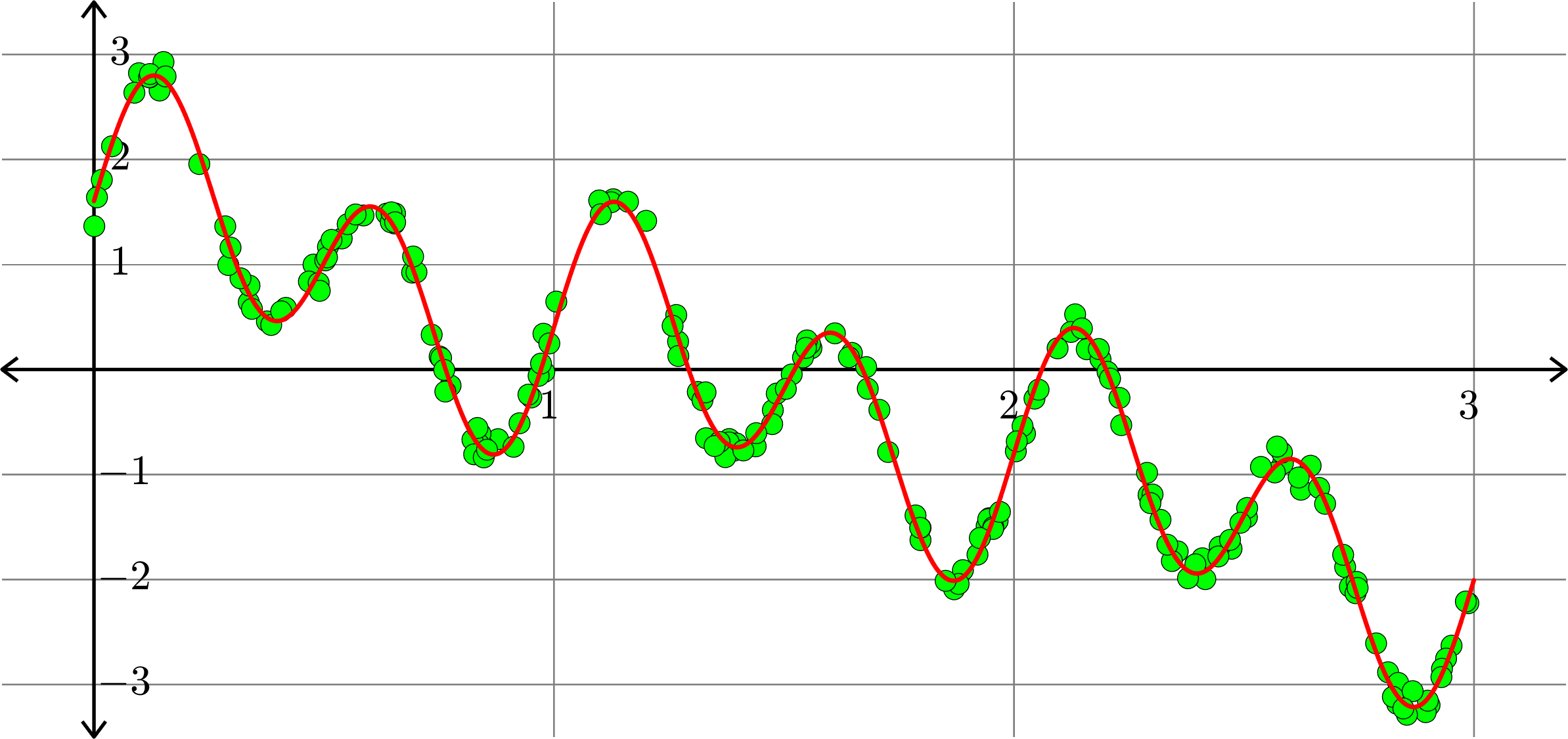
We want to find the function \(f\) of the form \[f(x) = a_{0}+\sum_{k=1}^{m}a_{k}\cos(2k\pi x)+\sum_{k=1}^{m}b_{k}\sin(2k\pi x)\] so that \(\displaystyle{\sum_{i=1}^{n}|f(x_{i})-y_{i}|^{2}}\) is as small as possible.
Set
We wish to find the least squares solution to \(Ax=b\).
\[A= \begin{bmatrix}1 & \cos(2\pi x_{1}) & \sin(2\pi x_{1}) & \cos(4\pi x_{1}) & \sin(4\pi x_{1}) & \cdots & \cos(2m\pi x_{1}) & \sin(2m\pi x_{1})\\1 & \cos(2\pi x_{2}) & \sin(2\pi x_{2}) & \cos(4\pi x_{2}) & \sin(4\pi x_{2}) & \cdots & \cos(2m\pi x_{2}) & \sin(2m\pi x_{2})\\1 & \cos(2\pi x_{3}) & \sin(2\pi x_{3}) & \cos(4\pi x_{3}) & \sin(4\pi x_{3}) & \cdots & \cos(2m\pi x_{3}) & \sin(2m\pi x_{3})\\ \vdots & \vdots & \vdots & \vdots & \vdots & & \vdots & \vdots \\ 1 & \cos(2\pi x_{n}) & \sin(2\pi x_{n}) & \cos(4\pi x_{n}) & \sin(4\pi x_{n}) & \cdots & \cos(2m\pi x_{n}) & \sin(2m\pi x_{n})\end{bmatrix}\]
\[b= \begin{bmatrix}y_{1} & y_{2} & y_{3} & \cdots & y_{n}\end{bmatrix}^{\top}\]
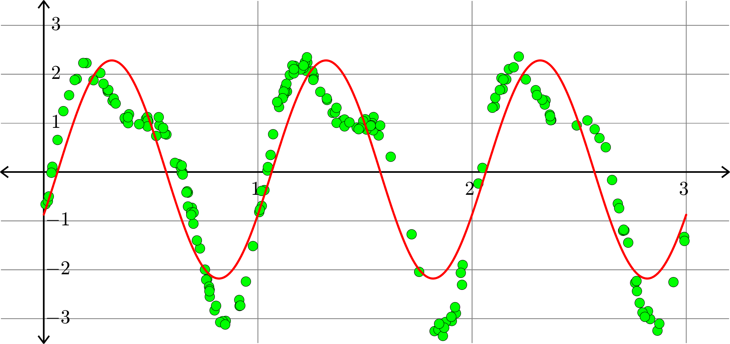
\[f(x)=0.0515-0.9225\cos(2\pi x)+2.0311\sin(2\pi x)\]
\[f(x) = -0.0058-1.0120\cos(2\pi x)+2.0076\sin(2\pi x)\]
\[-0.0074\cos(4\pi x)+0.9959\sin(4\pi x)\]
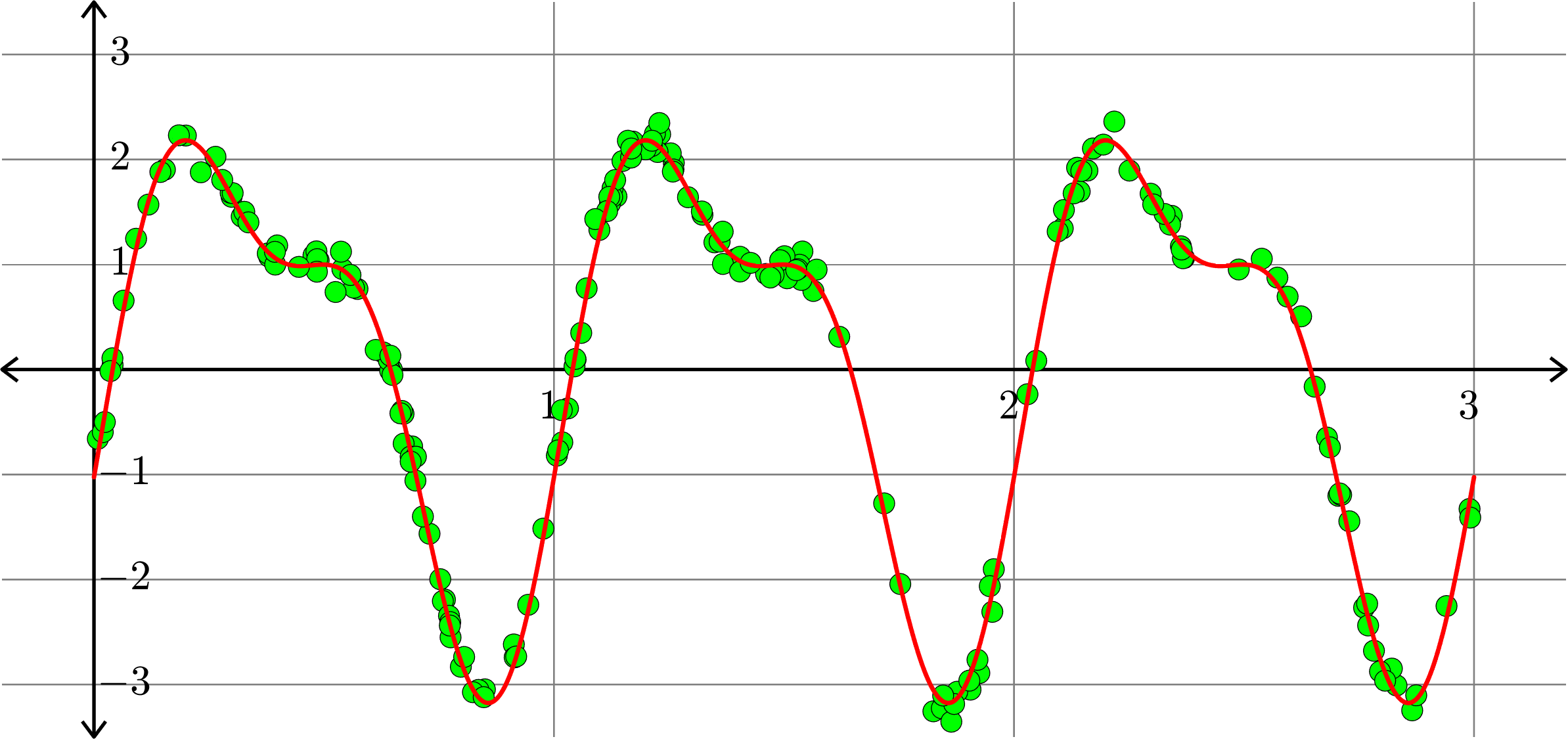
\[f(x) = -0.0055-1.0111\cos(2\pi x)+2.0075\sin(2\pi x)-0.0073\cos(4\pi x)\]
\[+0.9968\sin(4\pi x) + 0.0081\cos(6\pi x) - 0.0043\sin(6\pi x)\]

Fitting trigonometric polynomials
Consider the collection of points in \(\R^{2}\):
\[(x_{1},y_{1}),(x_{2},y_{2}),\ldots,(x_{n},y_{n})\]
Given a collection of functions \(f_{1},f_{2},\ldots,f_{m},\) we want to find the function \(f\) of the form \[f(x) = \sum_{k=1}^{m}a_{k}f_{k}(x)\] so that \(\displaystyle{\sum_{i=1}^{n}|f(x_{i})-y_{i}|^{2}}\) is as small as possible.
Set
We wish to find the least squares solution to \(Ax=b\).
\[A= \begin{bmatrix}f_{1}(x_{1}) & f_{2}(x_{1}) & f_{3}(x_{1}) & \cdots & f_{m}(x_{1})\\ f_{1}(x_{2}) & f_{2}(x_{2}) & f_{3}(x_{2}) & \cdots & f_{m}(x_{2})\\ f_{1}(x_{3}) & f_{2}(x_{3}) & f_{3}(x_{3}) & \cdots & f_{m}(x_{3})\\ \vdots & \vdots & \vdots & & \vdots\\ f_{1}(x_{n}) & f_{2}(x_{n}) & f_{3}(x_{n}) & \cdots & f_{m}(x_{n})\end{bmatrix} \quad\text{and}\quad b=\begin{bmatrix}y_{1}\\ y_{2}\\ y_{3}\\ \vdots\\ y_{n}\end{bmatrix}\]
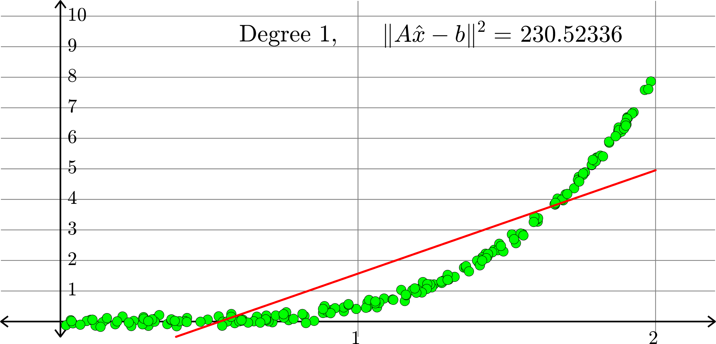
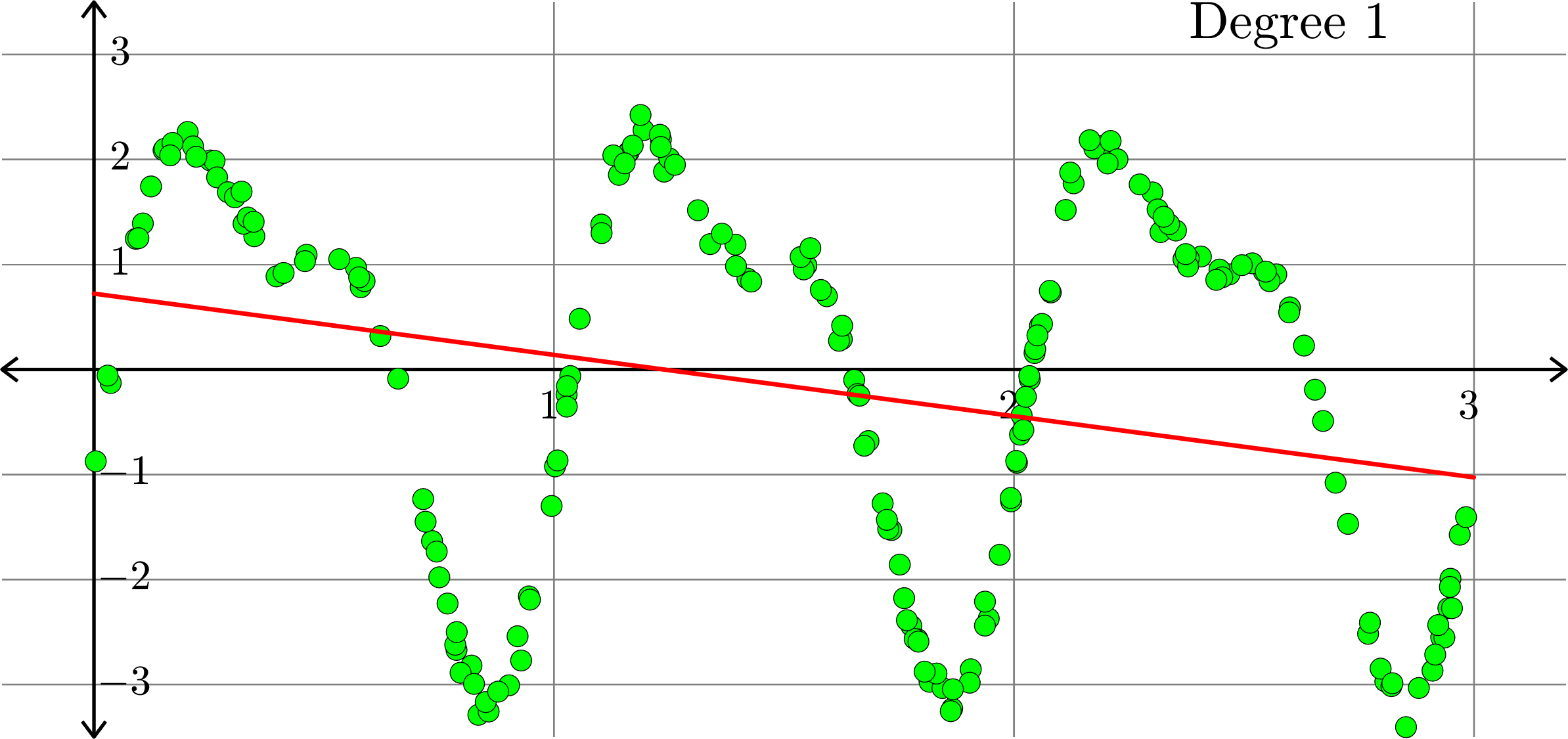
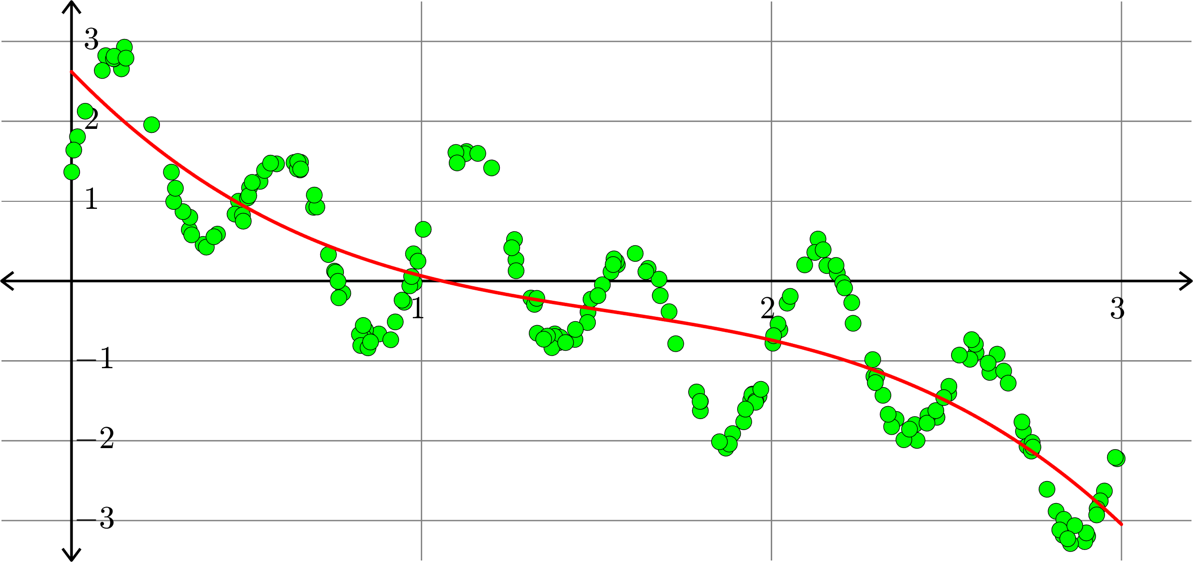
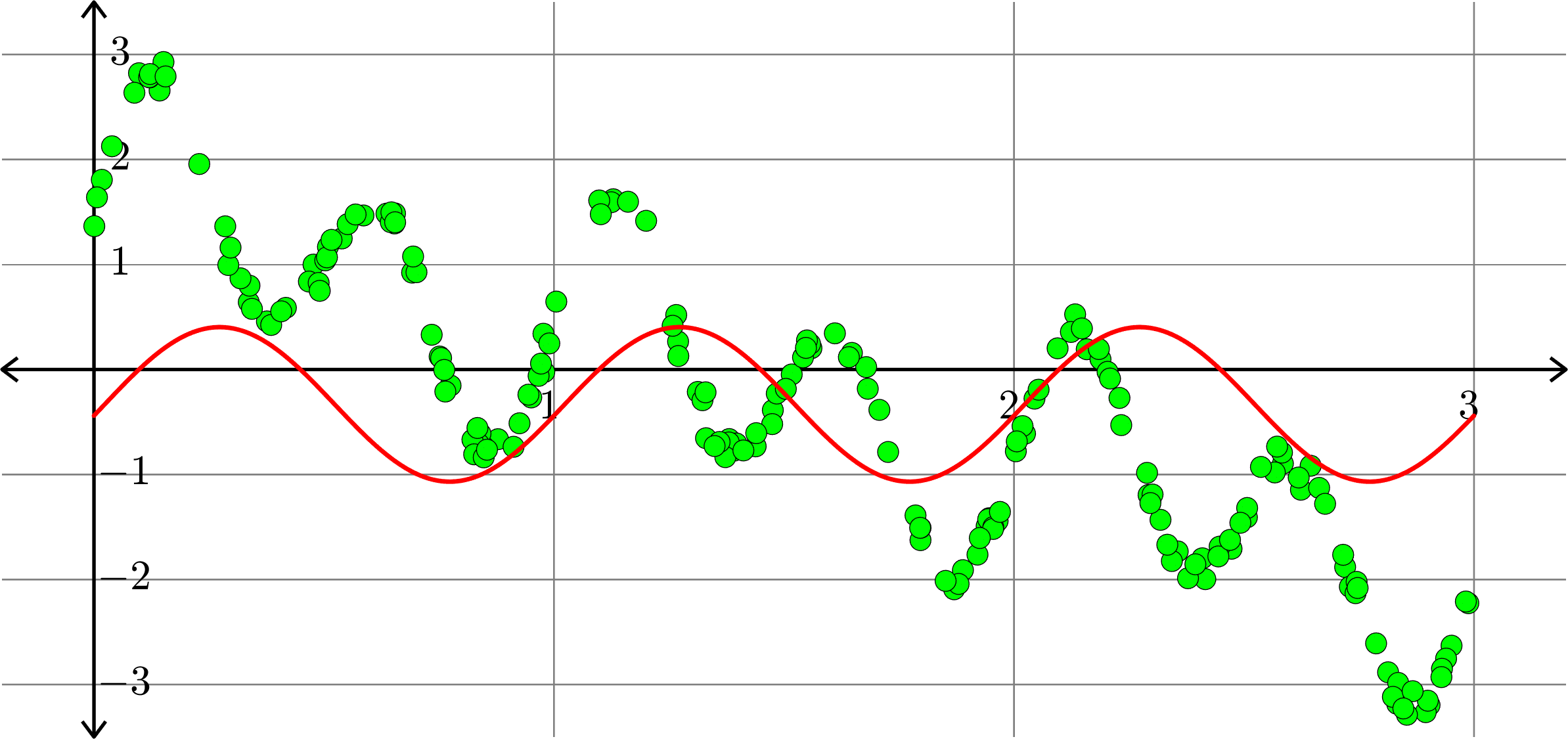
Polynomials and trig alone don't work:

Best fit function of the form:
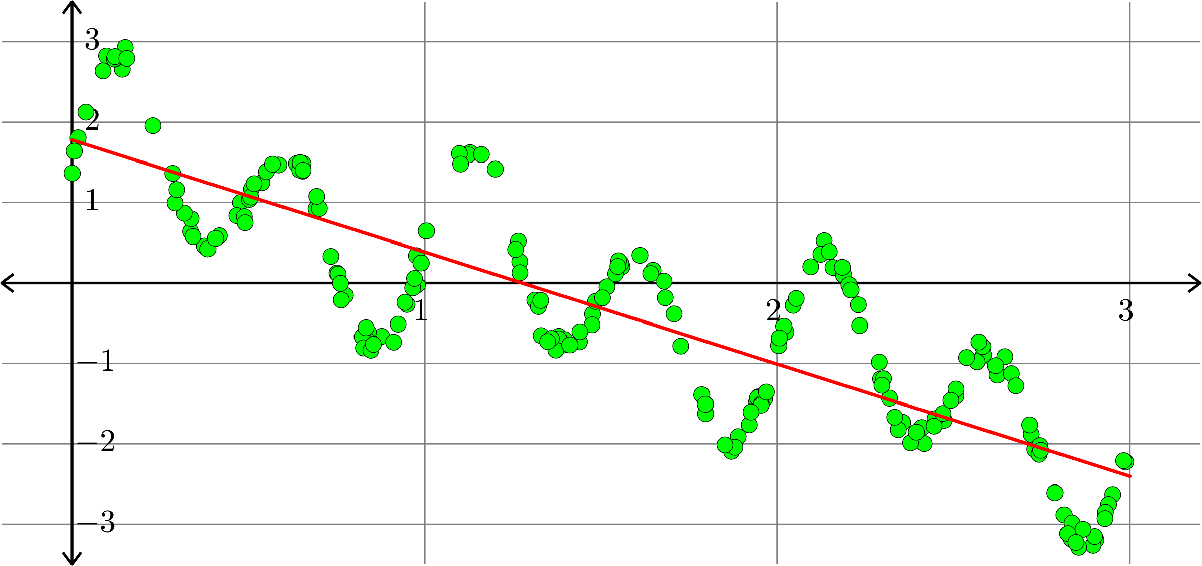
\(\displaystyle{f(x) = a_{0}+a_{1}x}\)
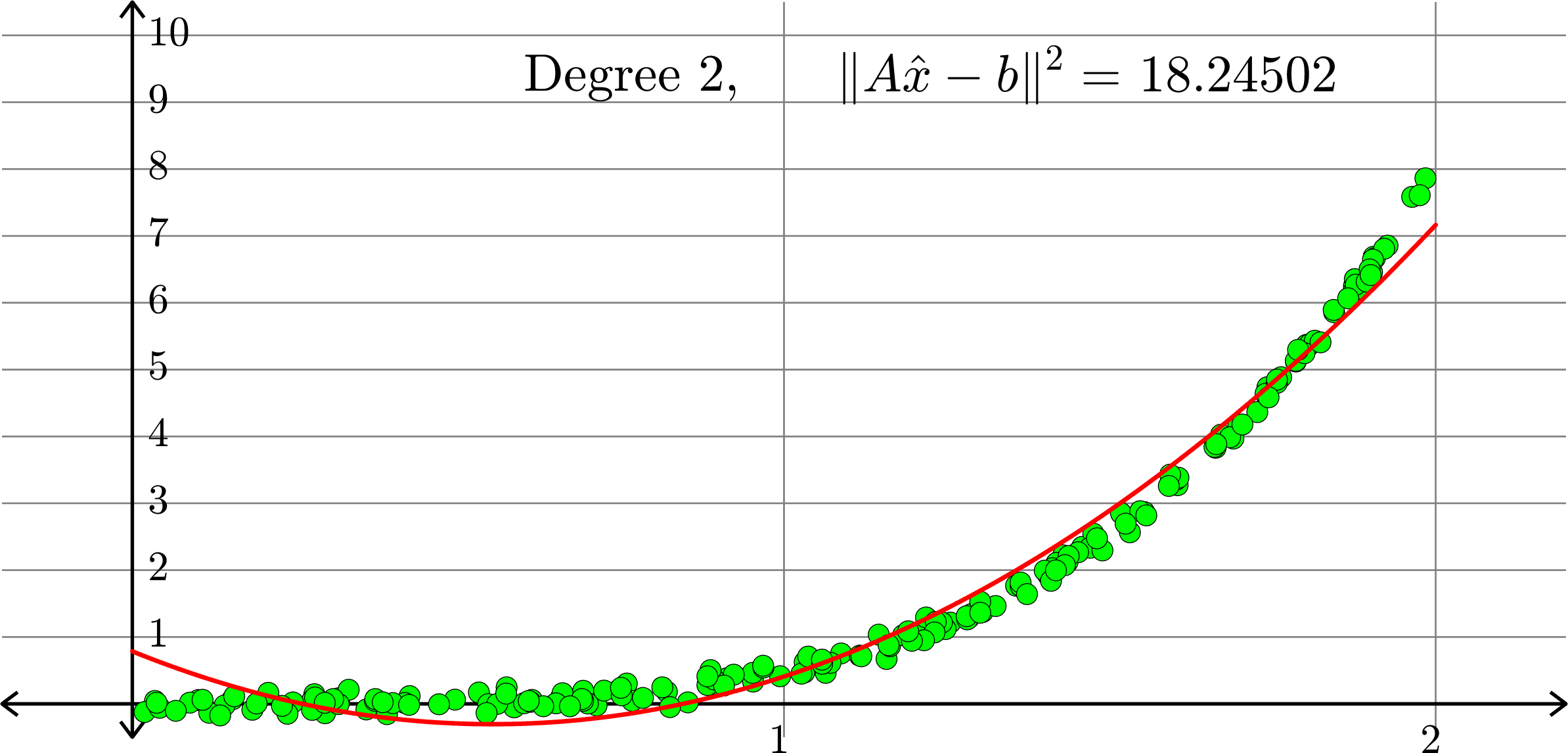
Polynomials and trig alone don't work:
Best fit function of the form:
\(\displaystyle{f(x) = a_{0}+a_{1}x+a_{2}x^2}\)

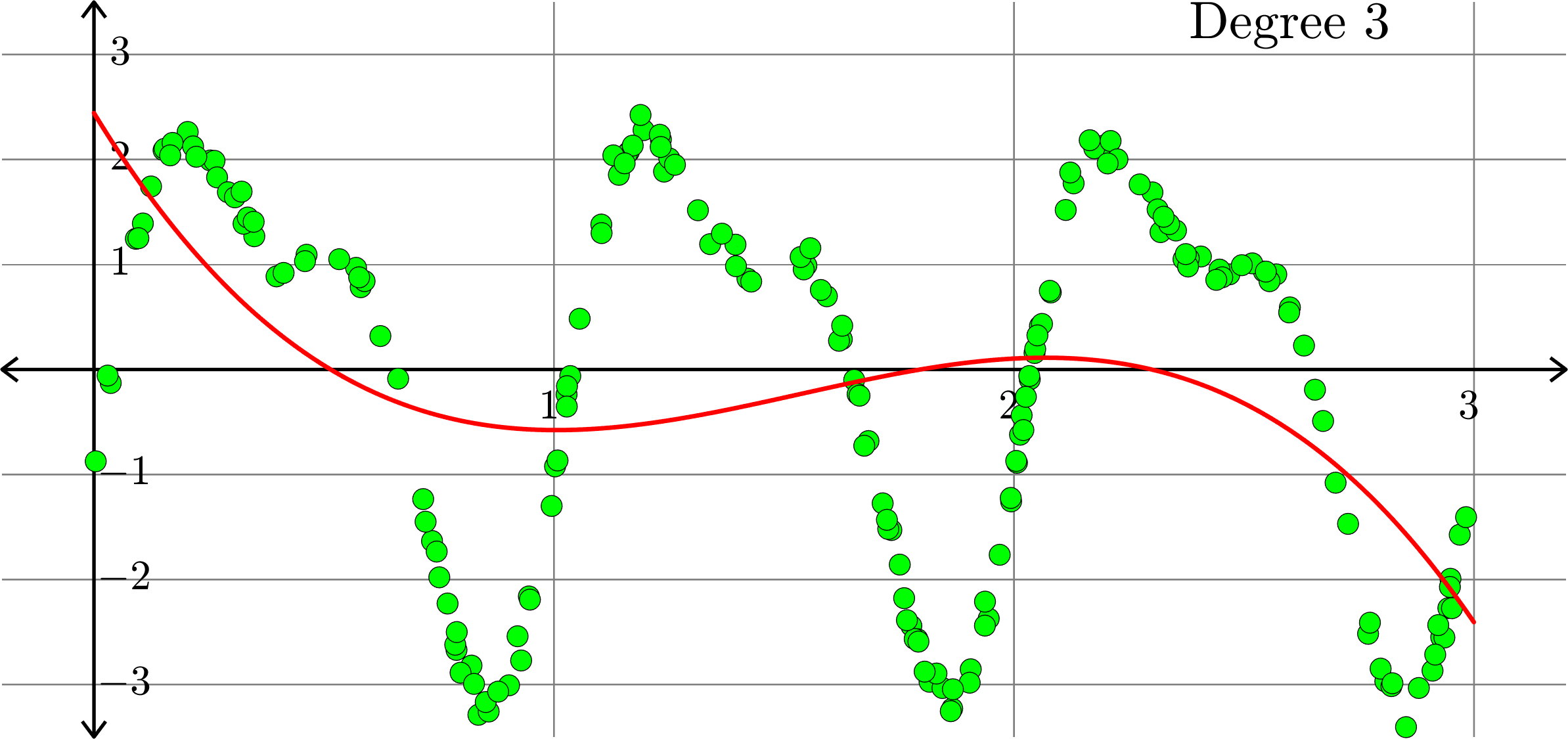
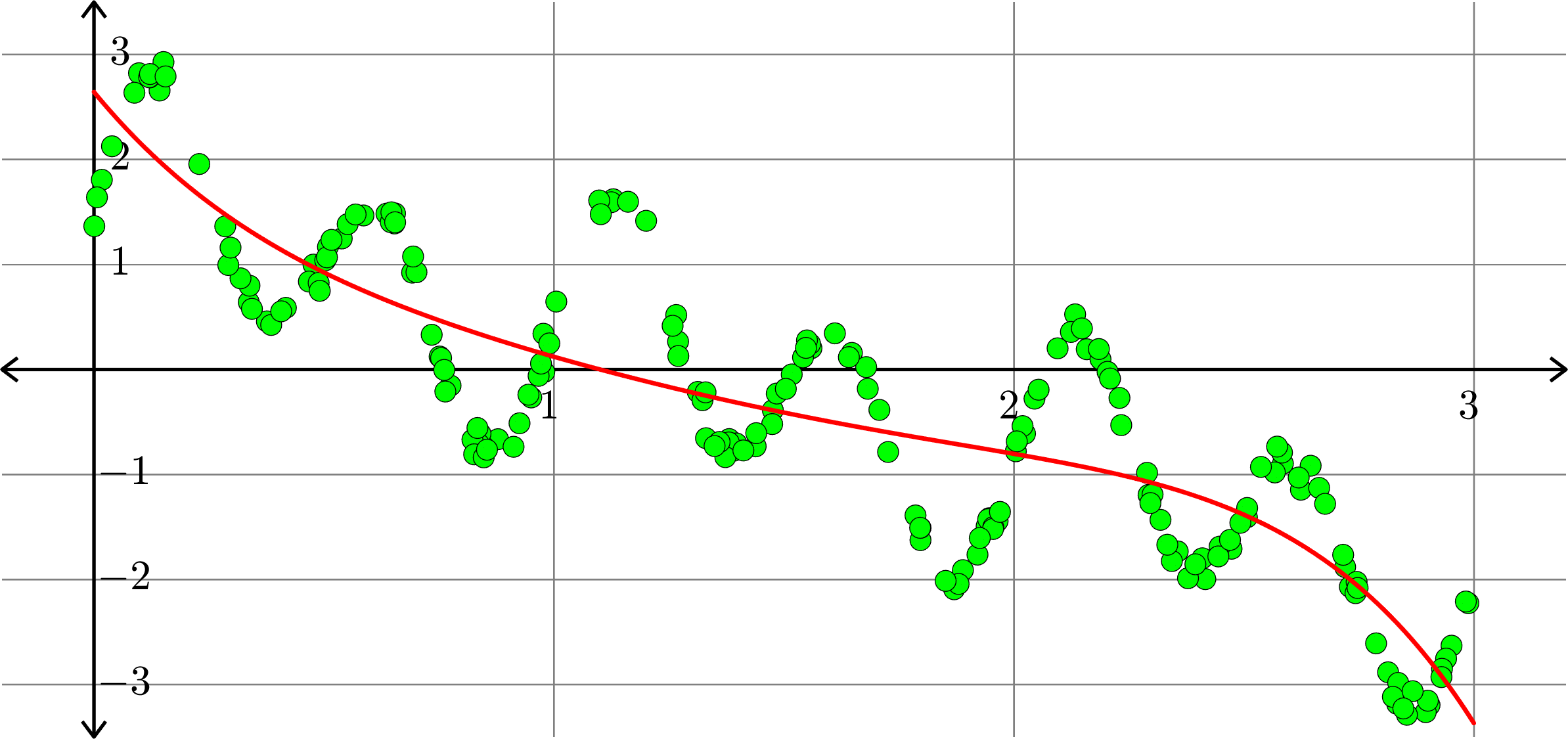
Polynomials and trig alone don't work:
Best fit function of the form:
\(\displaystyle{f(x) = a_{0}+a_{1}x+a_{2}x^2+a_{3}x^{3}}\)
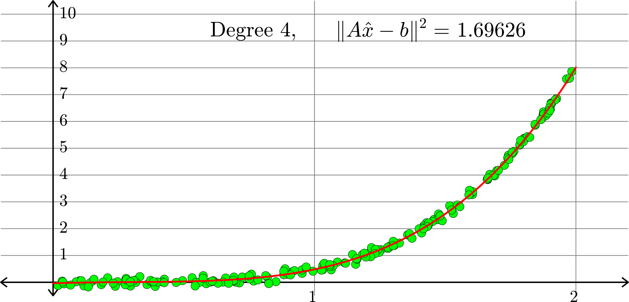
Polynomials and trig alone don't work:
Best fit function of the form:
\(\displaystyle{f(x) = a_{0}+a_{1}x+a_{2}x^2+a_{3}x^{3}+a_{4}x^4}\)

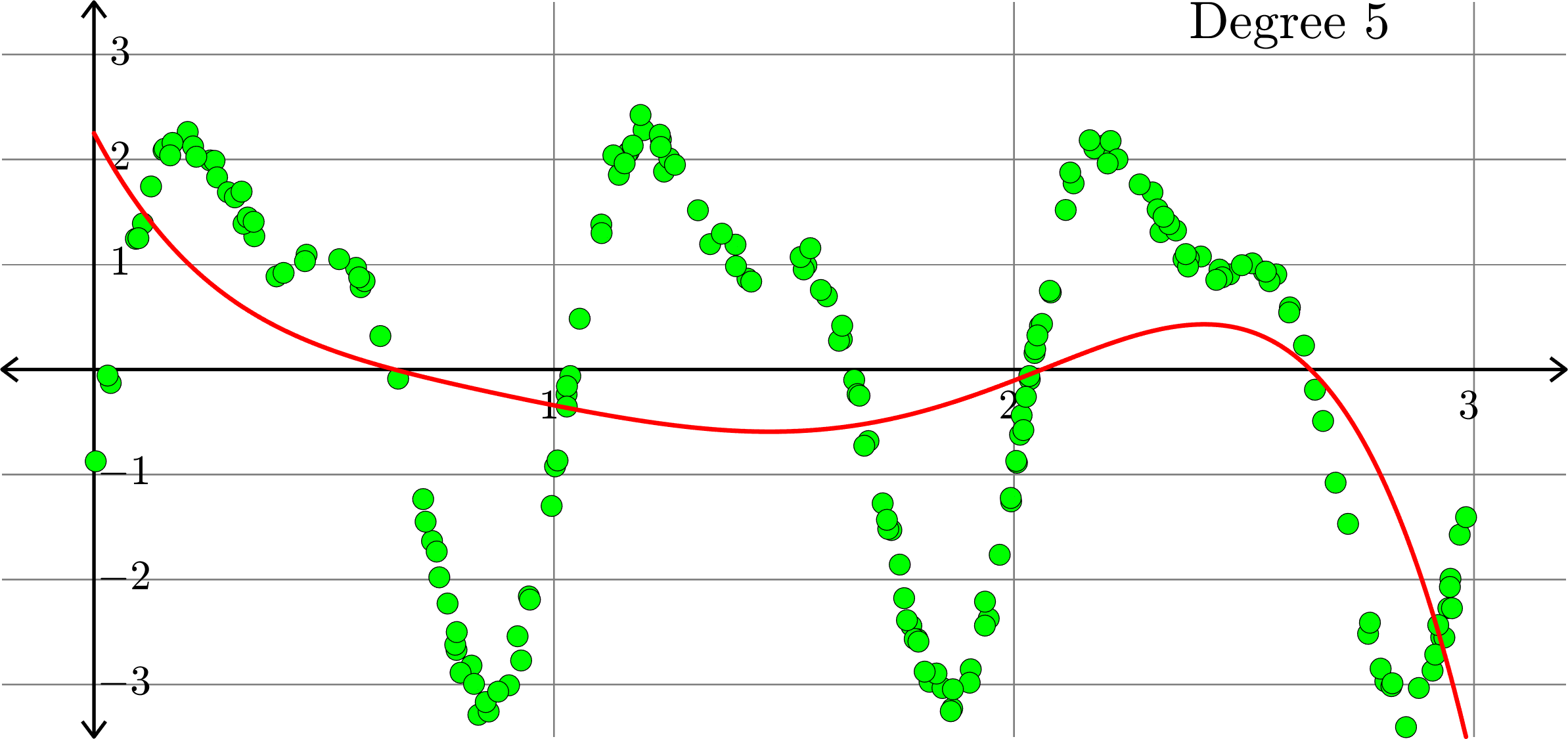
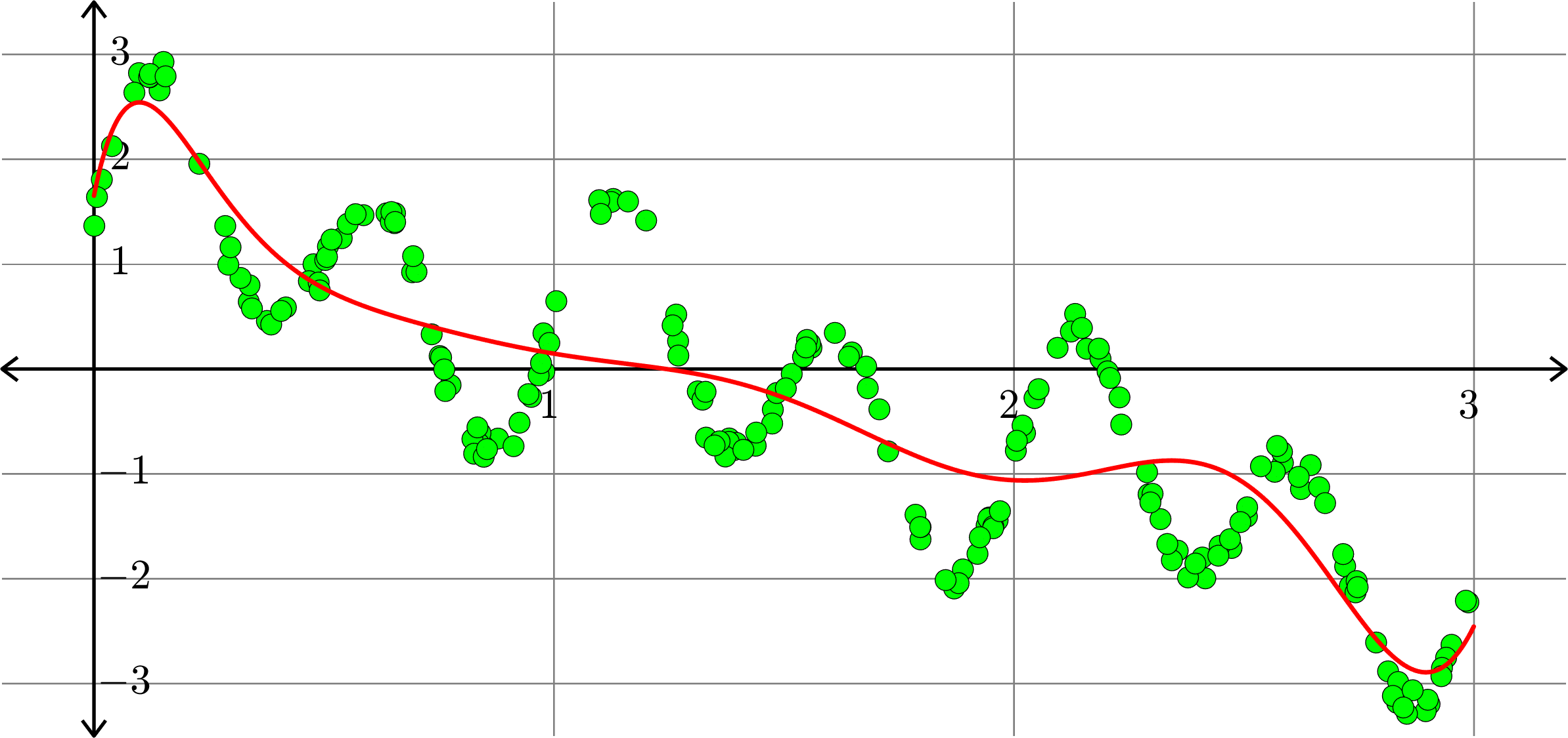
Polynomials and trig alone don't work:
Best fit function of the form:
\(\displaystyle{f(x) = \sum_{k=0}^{5}a_{k}x^k}\)
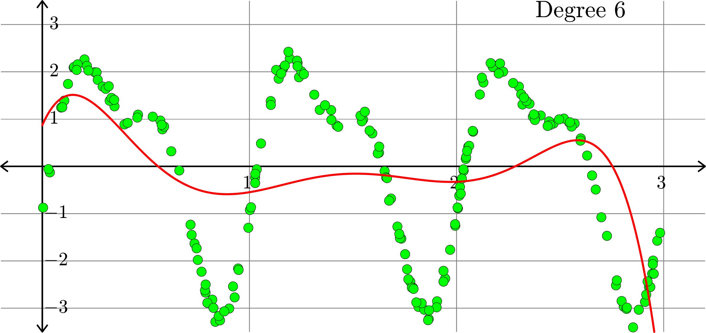
Polynomials and trig alone don't work:
Best fit function of the form:
\(\displaystyle{f(x) = \sum_{k=0}^{10}a_{k}x^k}\)
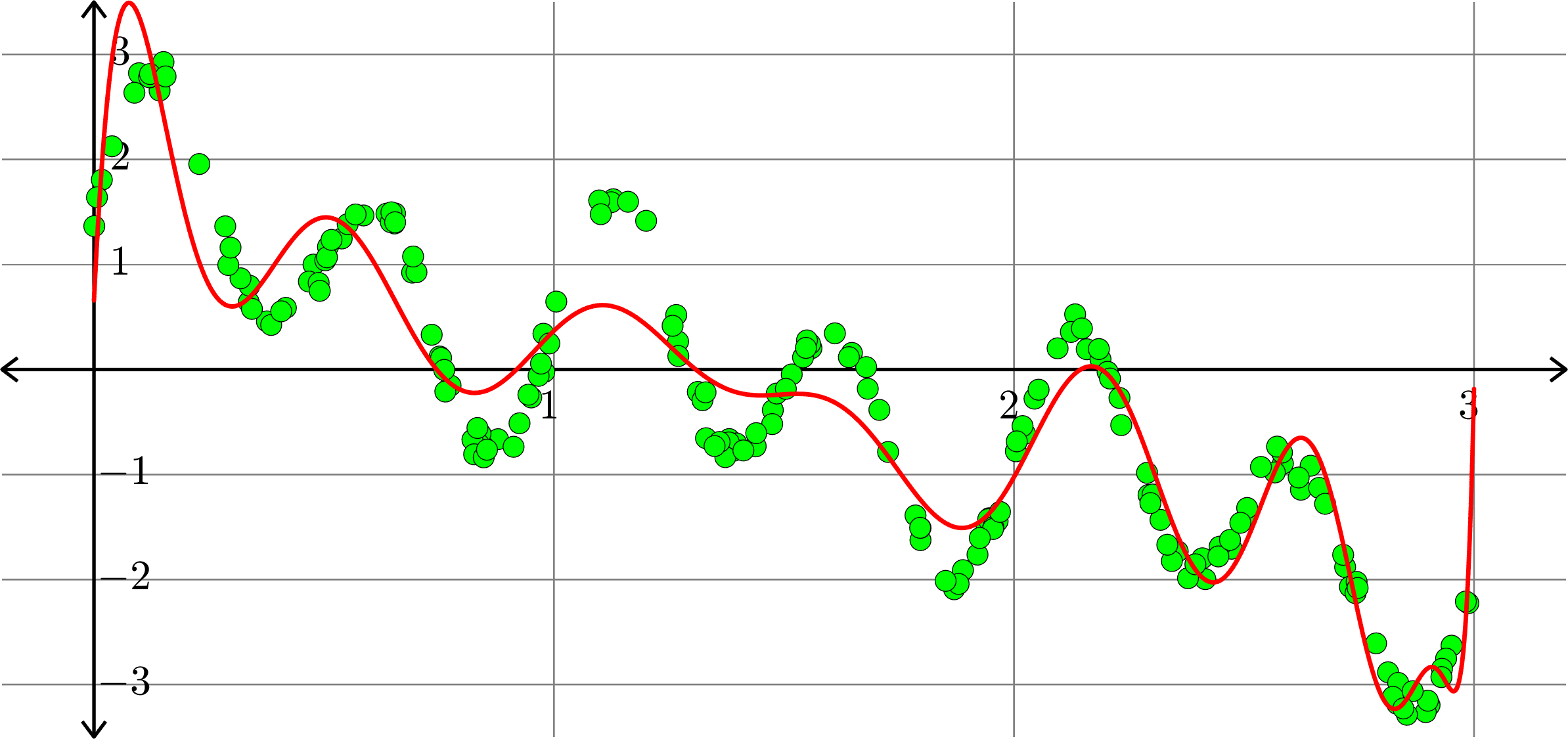
Polynomials and trig alone don't work:
Best fit function of the form:
\(\displaystyle{f(x) = \sum_{k=0}^{20}a_{k}x^k}\)
Polynomials and trig alone don't work:
Best fit function of the form:
\[f(x) = a_{0} + a_{1}\cos(2\pi x)+b_{1}\sin(2\pi x)\]
Polynomials and trig alone don't work:
Best fit function of the form:
\[f(x) = a_{0} + a_{1}\cos(2\pi x)+b_{1}\sin(2\pi x)+ a_{2}\cos(4\pi x)+b_{2}\sin(4\pi x)\]
Polynomials and trig alone don't work:
Best fit function of the form:
\[f(x) = a_{0} + \sum_{k=1}^{3}\big(a_{k}\cos(2k\pi x)+b_{k}\sin(2k\pi x)\big)\]
Polynomials and trig alone don't work:
Best fit function of the form:
\[f(x) = a_{0} + \sum_{k=1}^{4}\big(a_{k}\cos(2k\pi x)+b_{k}\sin(2k\pi x)\big)\]

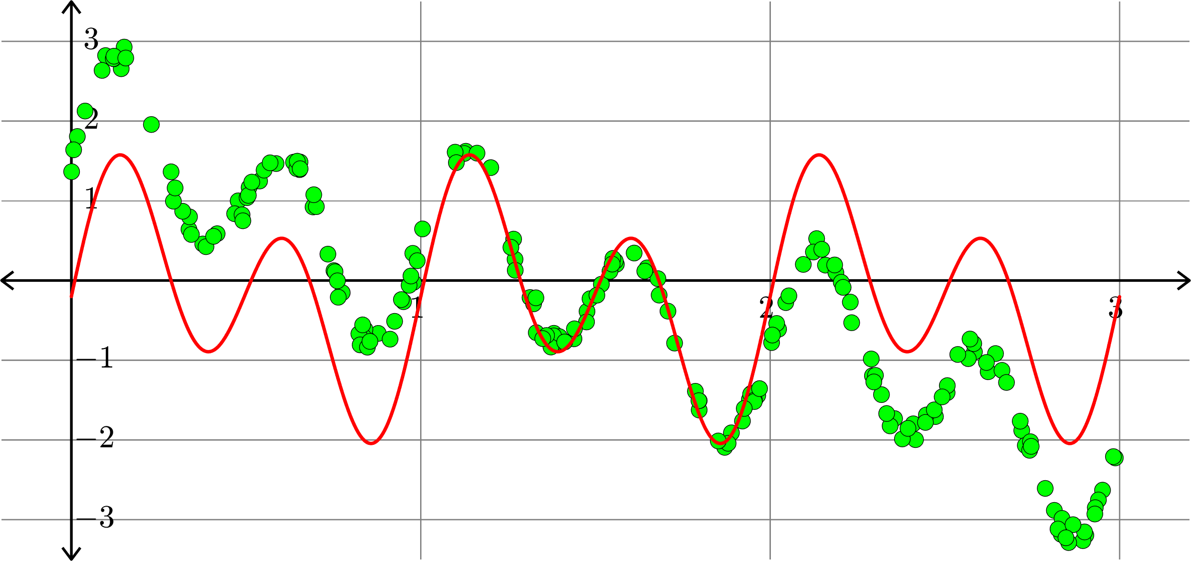
Polynomials and trig alone don't work:
Best fit function of the form:
\[f(x) = a_{0} + \sum_{k=1}^{5}\big(a_{k}\cos(2k\pi x)+b_{k}\sin(2k\pi x)\big)\]

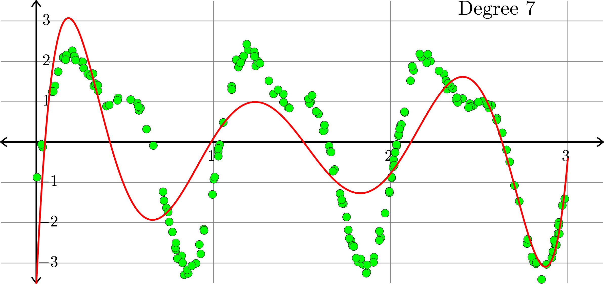
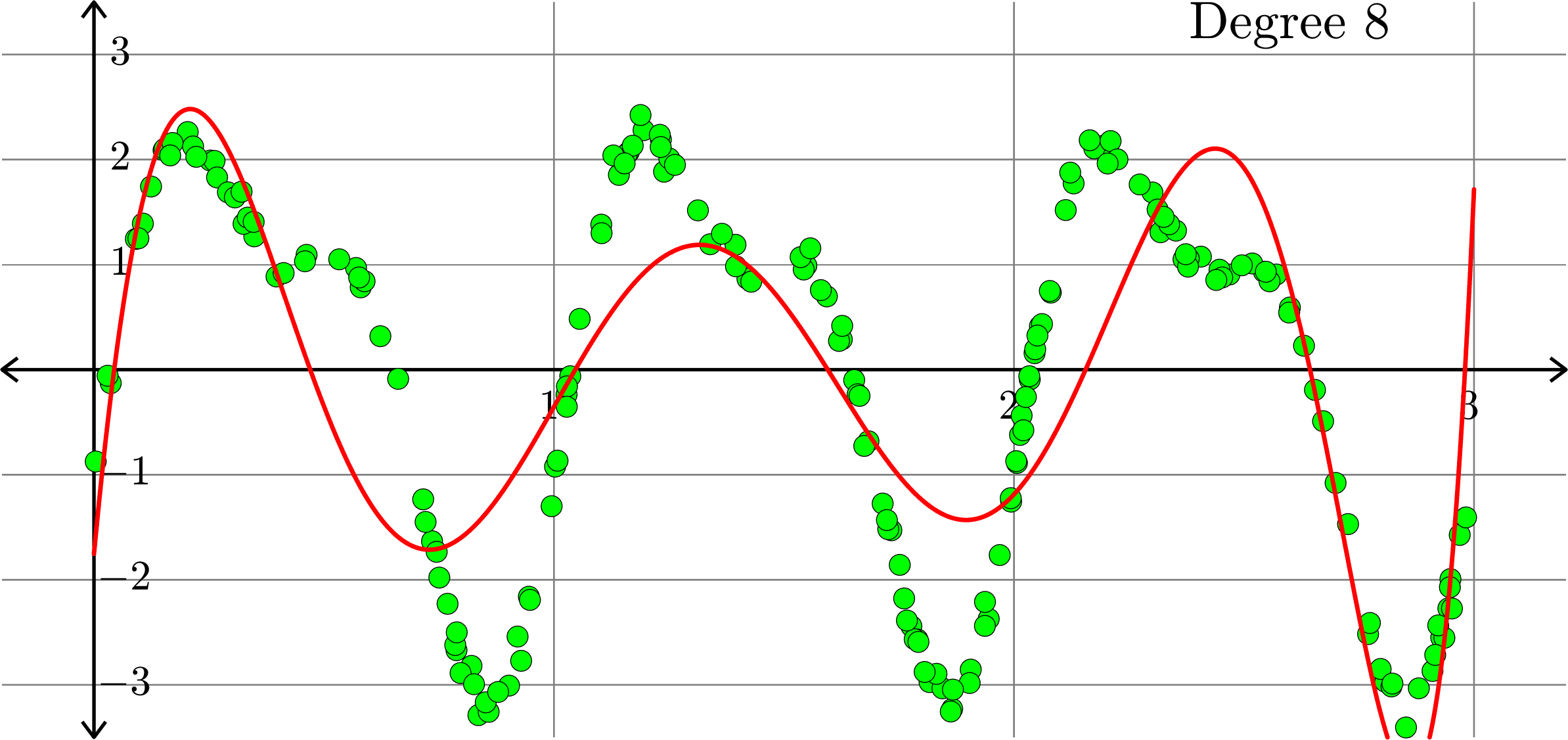
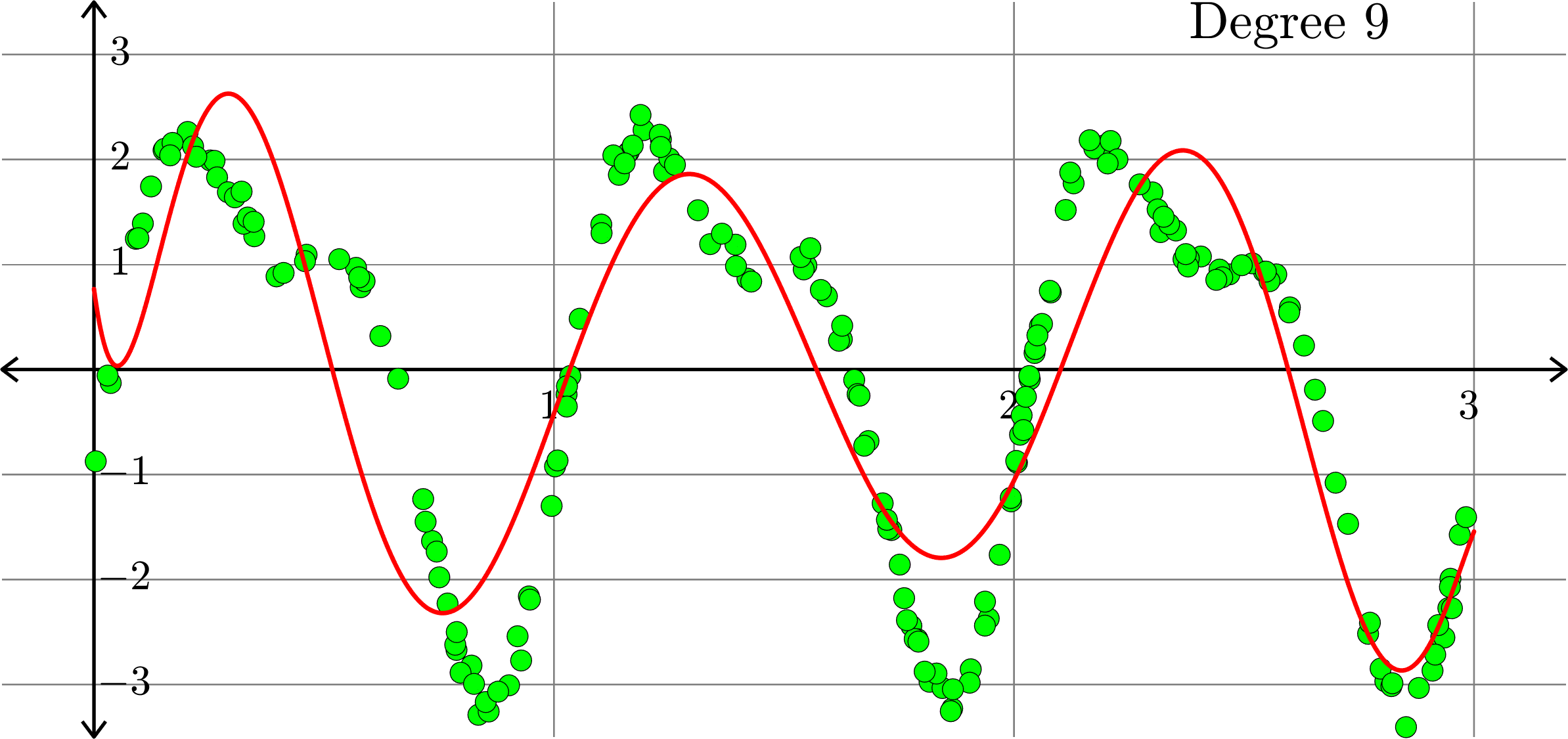
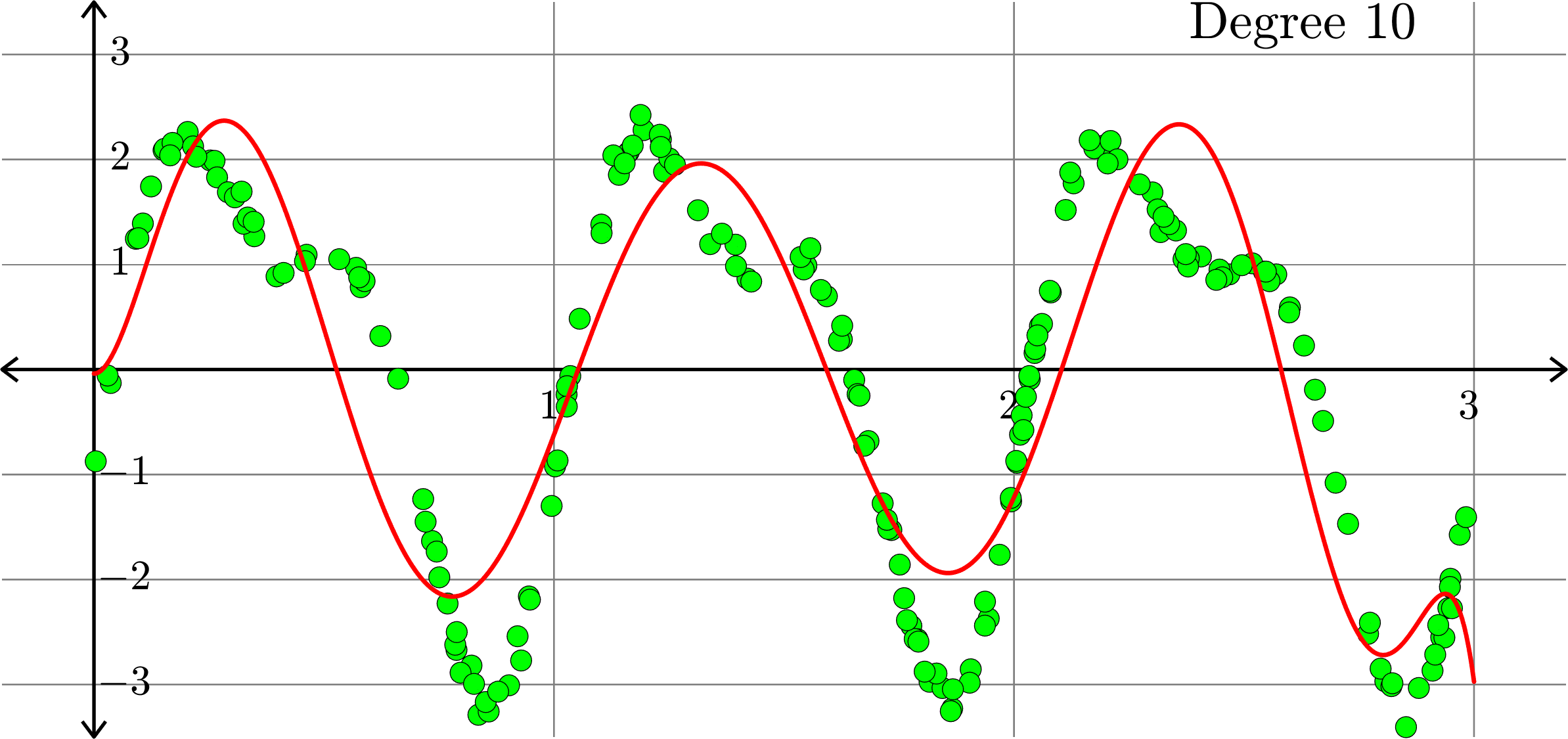
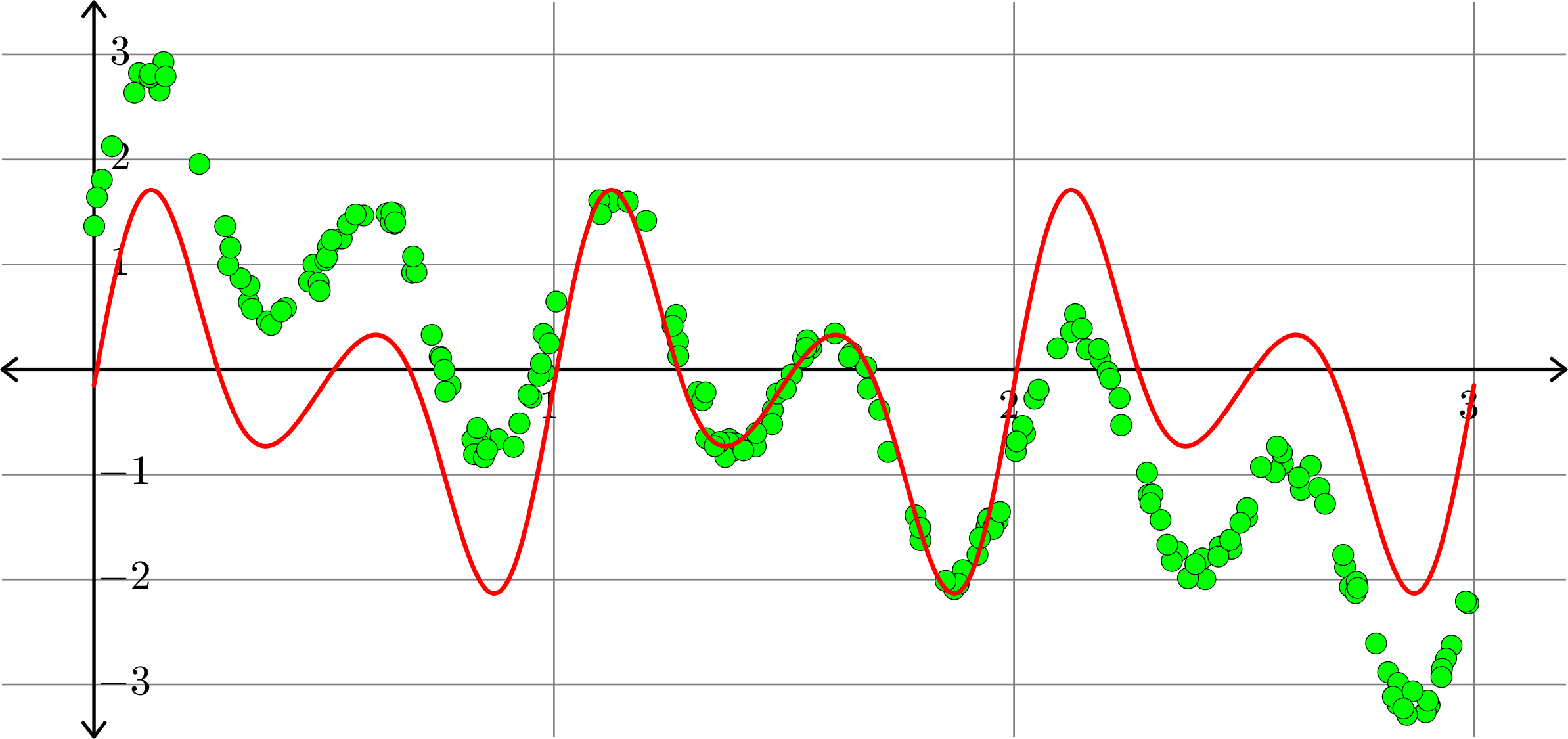
Polynomials and trig alone don't work:
Best fit function of the form:
\[f(x) = a_{0} + \sum_{k=1}^{10}\big(a_{k}\cos(2k\pi x)+b_{k}\sin(2k\pi x)\big)\]
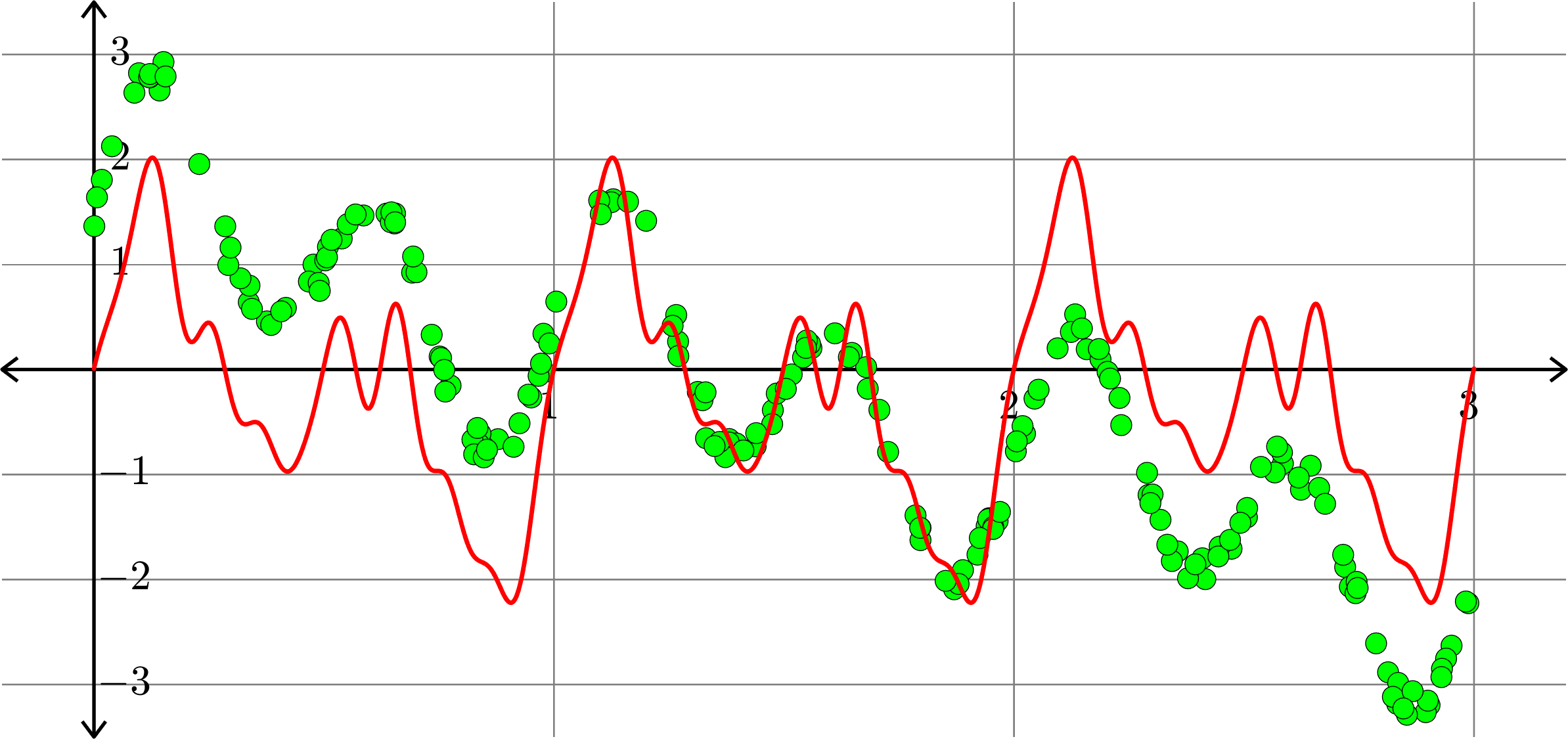
Polynomials and trig alone don't work:
Best fit function of the form:
\[f(x) = a_{0} + c_{1}x + a_{1}\cos(2\pi x)+b_{1}\sin(2\pi x)+ a_{2}\cos(4\pi x)+b_{2}\sin(4\pi x)\]
Orthonormal bases
Thus, if \(\{v_{1},v_{2},\ldots,v_{n}\}\) is an ONB for \(\R^{n}\), then
\[v = \sum_{i=1}^{n}(v_{i}\cdot v) v_{i}.\]
If \(I\subset \{1,2,\ldots,n\}\), then we define
\[v_{I} = \sum_{i\in I}(v_{i}\cdot v) v_{i}\]
and
\[\|v-v_{I}\|^{2} = \left\|\sum_{i=1}^{n}(v_{i}\cdot v)v_{i} - \sum_{i\in I}(v_{i}\cdot v)v_{i}\right\|^{2} = \Bigg\|\sum_{i\notin I}(v_{i}\cdot v)v_{i}\Bigg\|^{2} =\sum_{i\notin I}|v_{i}\cdot v|^{2}\]
In particular, let \(I\subset \{1,2,\ldots,n\}\) be the \(k\) indices \(i\) such that \(|v_{i}\cdot v|\) are largest. Then \(\|v-v_{I}\|\) is as small as possible among all sets \(I\).
Orthonormal bases
The set \(\{v_{1},v_{2},v_{3},v_{4}\}\) where
\[v_{1} = \frac{1}{2}\begin{bmatrix} 1\\ 1\\ 1\\ 1\end{bmatrix},\ v_{2} = \frac{1}{2}\begin{bmatrix} \phantom{-}1\\ -1\\ \phantom{-}1\\ -1\end{bmatrix},\ v_{3} = \frac{1}{2}\begin{bmatrix} \phantom{-}1\\ \phantom{-}1\\ -1\\ -1\end{bmatrix},\ v_{4} = \frac{1}{2}\begin{bmatrix} \phantom{-}1\\ -1\\ -1\\ \phantom{-}1\end{bmatrix},\]
is an orthonormal basis for \(\R^{4}\). We see that
\(v = \begin{bmatrix} 1\\ 1\\ 2\\ 4 \end{bmatrix} = 4v_{1} - v_{2}-2v_{3}+v_{4}\)
\[ = 4\left(\frac{1}{2}\begin{bmatrix} 1\\ 1\\ 1\\ 1\end{bmatrix}\right) + (-1)\left(\frac{1}{2}\begin{bmatrix} \phantom{-}1\\ -1\\ \phantom{-}1\\ -1\end{bmatrix}\right) + (-2)\left(\frac{1}{2} \begin{bmatrix} \phantom{-}1\\ \phantom{-}1\\ -1\\ -1\end{bmatrix}\right) + (1)\left(\frac{1}{2}\begin{bmatrix} \phantom{-}1\\ -1\\ -1\\ \phantom{-}1\end{bmatrix}\right)\]
Take \(I=\{1,3\}\) and we have \(\|v - v_{I}\| = \sqrt{2}\).
Orthonormal bases
To store the vector
\[v = \begin{bmatrix} 1\\ 1\\ 2\\ 4 \end{bmatrix} = 4v_{1} - v_{2}-2v_{3}+v_{4}\]
we need to store 4 numbers.
Instead, we store the approximation
\[v_{I} = 4v_{1} - 2v_{3} = \begin{bmatrix} 1\\ 1\\ 3\\ 3 \end{bmatrix}.\]
So, we only need to store TWO numbers \(4\) and \(-2\).
This is not quite true, why?
Image compression using a "nice" ONB
Thinking of an image as a large set of vectors
\[p_{1} = \begin{bmatrix} p_{11}\\ p_{21}\\ p_{31}\\ \vdots\\ p_{m1} \end{bmatrix},\ p_{2} = \begin{bmatrix} p_{12}\\ p_{22}\\ p_{32}\\ \vdots\\ p_{m2} \end{bmatrix},\ \ldots,\ p_{n} = \begin{bmatrix} p_{1n}\\ p_{2n}\\ p_{3n}\\ \vdots\\ p_{mn} \end{bmatrix}.\]
(Think of each "patch" as a vector.)
For each \(p_{j}\) we expand with respect to an ONB \(\{v_{1},\ldots,v_{m}\}\) and we have
Now, we throw away all but the \(k\) term with the largest coefficients (in absolute value), and we get our approximations:
\[p_{j}^{(k)} = \sum_{i\in I_{j}}(v_{i}\cdot p_{j})v_{i}\]
\[p_{j} = \sum_{i=1}^{m}(v_{i}\cdot p_{j}) v_{i}\]
Image compression using a "nice" ONB
In order to store
\[p_{j}^{(k)} = \sum_{i\in I_{j}}(v_{i}\cdot p_{j})v_{i}\]
We store the pairs \((v_{i}\cdot p_{j}, i)\) where \(i\in I\). Since \(I\) has \(k\) elements, this means that we are storing \(2k\) numbers.
Example. If
\[v = 10v_{1} - v_{2} + 6v_{3} +\frac{1}{3}v_{4} + \frac{1}{10}v_{5} - 14v_{6}+\frac{1}{2}v_{7} + v_{8} - \frac{2}{3}v_{9}+\frac{2}{5}v_{10}\]
Then, keeping the thee largest coefficients we get
\[v^{(3)} = 10v_{1}+ 6v_{3}- 14v_{6}\]
We store the pairs \((10,1), (6,3)\) and \((-14,6)\) and we can recover the approximation \(v^{(3)}\).
Linear Algebra Day 33
By John Jasper


