Simulation-Based Inference: estimating posterior distributions without analytic likelihoods
Rencontres Statistiques Lyonnaises, Villeurbanne, France
September 16, 2024
Justine Zeghal
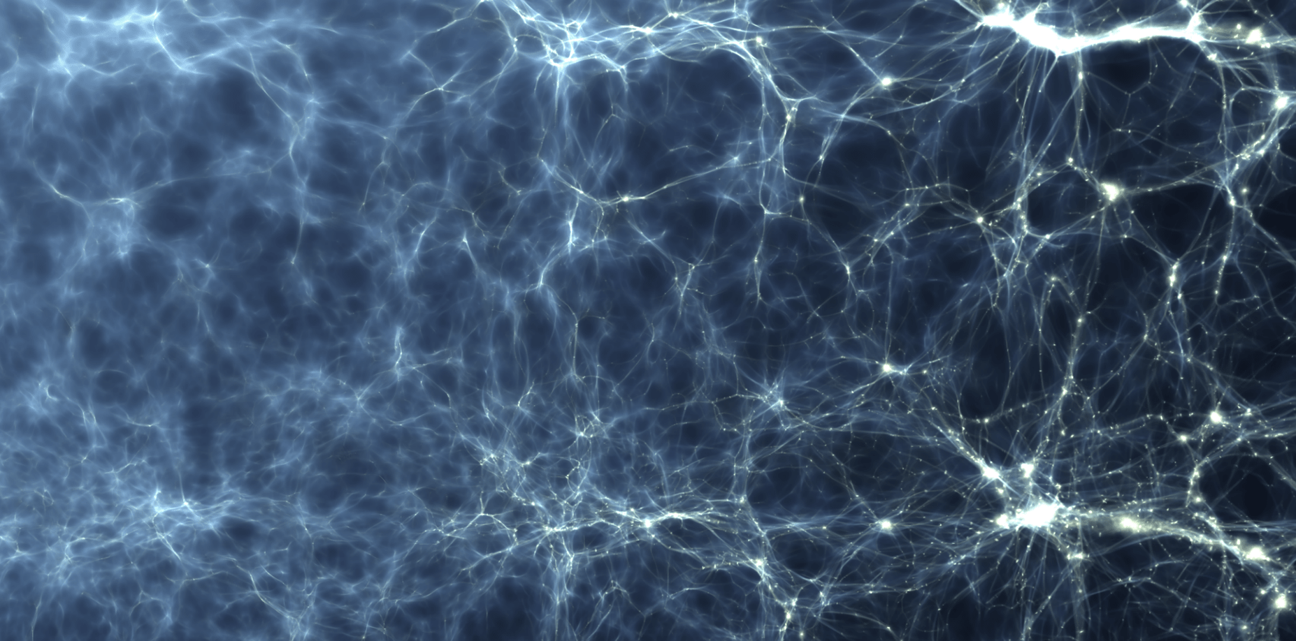


credit: Villasenor et al. 2023
Quick cosmological introduction
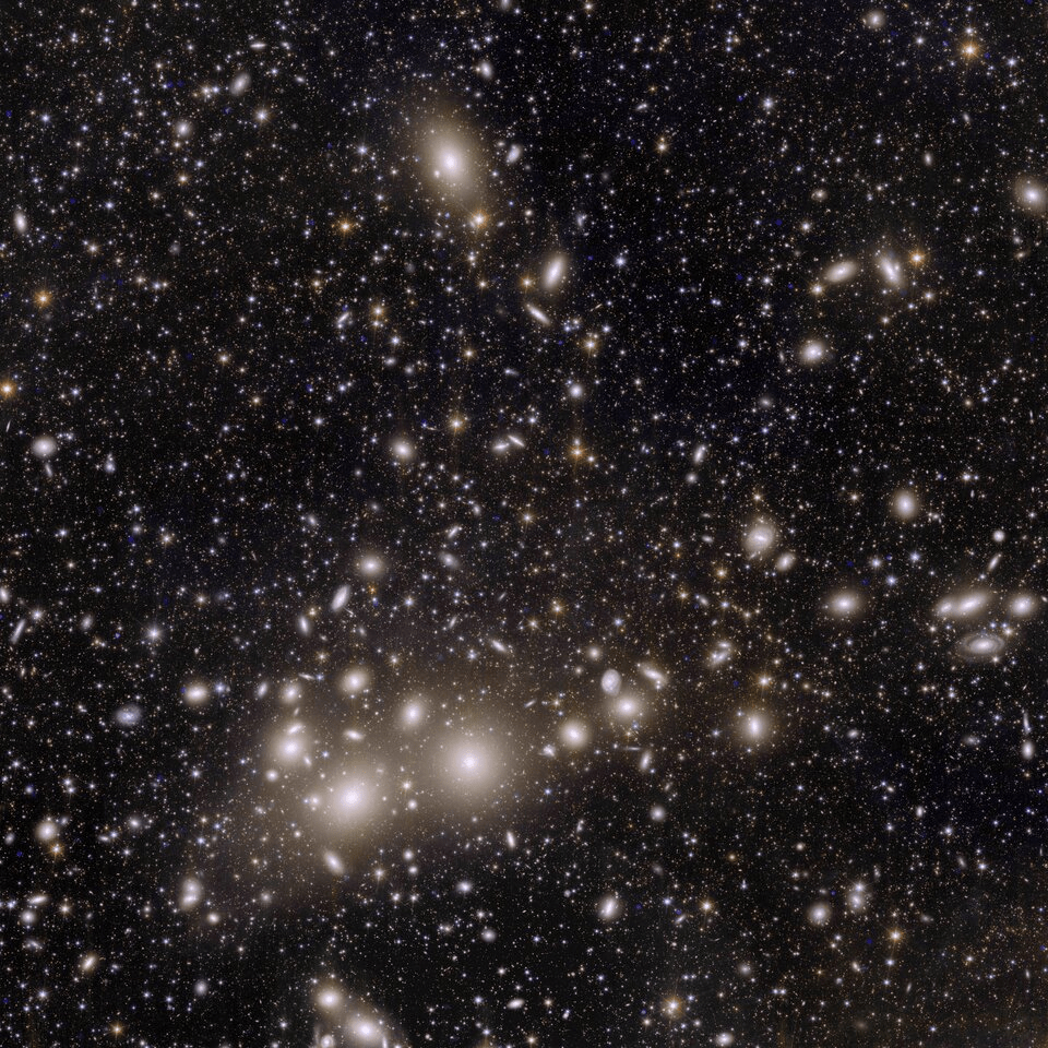
Credit: ESATo date, the model that best describes our observations is
\Lambda \text{CDM}
and it relies only on 6 cosmological parameters:
\Omega_c,\: \Omega_b,\: \sigma_8,\: n_s,\: w_0,\: h_0.
One big goal in cosmology is to determine the value of those parameters based on our observations.
Bayesian inference
\underbrace{p(\theta|x=x_0)}_{\text{posterior}}
\underbrace{p(\theta)}_{\text{prior}}
\underbrace{p(x = x_0|\theta)}_{\text{likelihood}}
\propto
Bayes theorem:
We want to infer the parameters that generated an observation
\theta
x_0
And run a MCMC to get the posterior
Bayesian inference
Cosmological context
\underbrace{p(\theta|x=x_0)}_{\text{posterior}}
\underbrace{p(\theta)}_{\text{prior}}
\underbrace{p(x = x_0|\theta)}_{\text{likelihood}}
\propto
Bayes theorem:
We want to infer the parameters that generated an observation
\theta
x_0
\underbrace{p(\theta|x=x_0)}_{\text{posterior}}
\underbrace{p(\theta)}_{\text{prior}}
\underbrace{p(x = x_0|\theta)}_{\text{likelihood}}
\propto
Bayes theorem:
\Omega_c\\ \Omega_b\\ \sigma_8\\ n_s\\ w_0\\ h_0
p(
|
)
x
Problem:
we do not have an analytic marginal likelihood that maps the cosmological parameters to what we observe
We want to infer the parameters that generated an observation
\theta
x_0
Credit: ESACosmological context
\underbrace{p(\theta|x=x_0)}_{\text{posterior}}
\underbrace{p(\theta)}_{\text{prior}}
\underbrace{p(x = x_0|\theta)}_{\text{likelihood}}
\propto
Bayes theorem:
\Omega_c\\ \Omega_b\\ \sigma_8\\ n_s\\ w_0\\ h_0
p(
|
)
x
Classical way of performing Bayesian Inference in Cosmology:
We want to infer the parameters that generated an observation
\theta
x_0
Credit: ESACosmological context
\underbrace{p(\theta|x=x_0)}_{\text{posterior}}
\underbrace{p(\theta)}_{\text{prior}}
\underbrace{p(x = x_0|\theta)}_{\text{likelihood}}
\propto
Bayes theorem:
\Omega_c\\ \Omega_b\\ \sigma_8\\ n_s\\ w_0\\ h_0
p(
|
)
We want to infer the parameters that generated an observation
\theta
x_0
Classical way of performing Bayesian Inference in Cosmology:
Power Spectrum
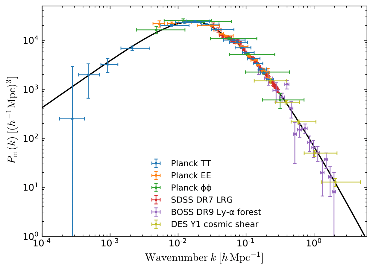
Credit: arxiv.org/abs/1807.06205Cosmological context
\underbrace{p(\theta|x=x_0)}_{\text{posterior}}
\underbrace{p(\theta)}_{\text{prior}}
\underbrace{p(x = x_0|\theta)}_{\text{likelihood}}
\propto
Bayes theorem:
\Omega_c\\ \Omega_b\\ \sigma_8\\ n_s\\ w_0\\ h_0
p(
|
)
We want to infer the parameters that generated an observation
\theta
x_0
Classical way of performing Bayesian Inference in Cosmology:
Power Spectrum
& Gaussian Likelihood
Cosmological context
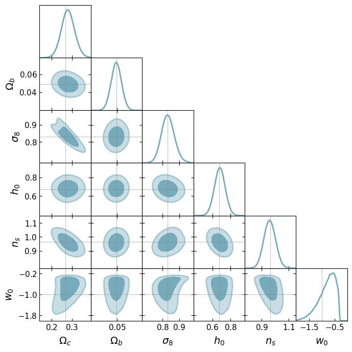
On large scales, the Universe is close to a Gaussian field and the 2-point function is a near sufficient statistic.
Cosmological context
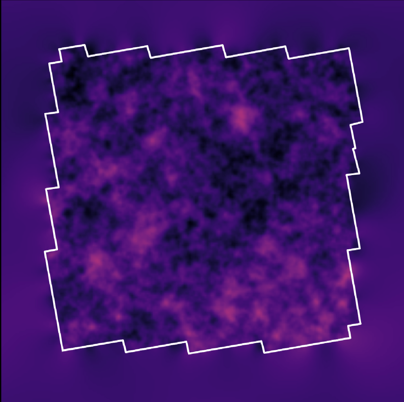
Credit: Benjamin RemyOn large scales, the Universe is close to a Gaussian field and the 2-point function is a near sufficient statistic.
Cosmological context
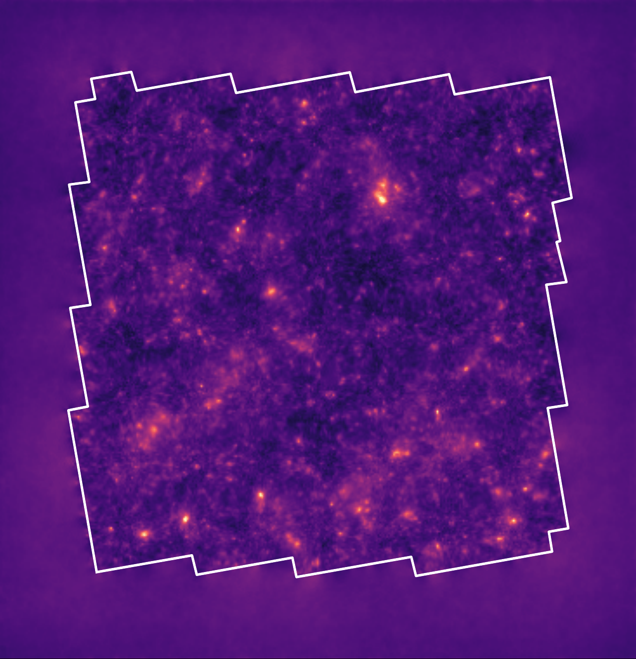
However, on small scales where non-linear evolution gives rise to a highly non-Gaussian field, this summary statistic is not sufficient anymore.
Credit: Benjamin RemyOn large scales, the Universe is close to a Gaussian field and the 2-point function is a near sufficient statistic.
However, on small scales where non-linear evolution gives rise to a highly non-Gaussian field, this summary statistic is not sufficient anymore.
Proof: full-field inference yield tighter constrain.
Cosmological context
How to do full-field inference?
\underbrace{p(\theta|x=x_0)}_{\text{posterior}}
\underbrace{p(\theta)}_{\text{prior}}
\underbrace{p(x = x_0|\theta)}_{\text{likelihood}}
\propto
Bayes theorem:
How to do full-field inference?
\underbrace{p(\theta|x=x_0)}_{\text{posterior}}
\underbrace{p(\theta)}_{\text{prior}}
\underbrace{p(x = x_0|\theta)}_{\text{likelihood}}
\propto
Bayes theorem:
How to do full-field inference?
\underbrace{p(\theta|x=x_0)}_{\text{posterior}}
\underbrace{p(\theta)}_{\text{prior}}
\underbrace{p(x = x_0|\theta)}_{\text{likelihood}}
\propto
Bayes theorem:
We can build a simulator to map the cosmological parameters to the data.
Simulator
How to do full-field inference?
\underbrace{p(\theta|x=x_0)}_{\text{posterior}}
\underbrace{p(\theta)}_{\text{prior}}
\underbrace{p(x = x_0|\theta)}_{\text{likelihood}}
\propto
Bayes theorem:
We can build a simulator to map the cosmological parameters to the data.
\theta
Simulator
How to do full-field inference?
\underbrace{p(\theta|x=x_0)}_{\text{posterior}}
\underbrace{p(\theta)}_{\text{prior}}
\underbrace{p(x = x_0|\theta)}_{\text{likelihood}}
\propto
Bayes theorem:
We can build a simulator to map the cosmological parameters to the data.
x
\theta
Simulator
How to do full-field inference?
\underbrace{p(\theta|x=x_0)}_{\text{posterior}}
\underbrace{p(\theta)}_{\text{prior}}
\underbrace{p(x = x_0|\theta)}_{\text{likelihood}}
\propto
Bayes theorem:
We can build a simulator to map the cosmological parameters to the data.
Prediction
x
\theta
Simulator
How to do full-field inference?
\underbrace{p(\theta|x=x_0)}_{\text{posterior}}
\underbrace{p(\theta)}_{\text{prior}}
\underbrace{p(x = x_0|\theta)}_{\text{likelihood}}
\propto
Bayes theorem:
We can build a simulator to map the cosmological parameters to the data.
Prediction
x
\theta
Simulator
Inference
How to do full-field inference?
How to do inference?
x
\theta
Simulator
How to do inference?
z
f
Depending on the simulator’s nature we can either perform
- Explicit inference
- Implicit inference
x
\theta
Simulator
Explicit inference
Explicit joint likelihood
p(x| \theta, z)
p(x| \theta, z)
\sigma^2
\mathcal{N}
z
f
x
\theta
Explicit simulator
Explicit inference
Explicit joint likelihood
p(x| \theta, z)
\sigma^2
\mathcal{N}
z
f
x
\theta
Explicit simulator
p(\theta, z \: | \: x) \propto
p(z\:|\:\theta) p(\theta)
Needs an explicit simulator to sample the joint posterior through MCMC:
p(x| \theta, z)
Explicit inference
Explicit joint likelihood
p(x| \theta, z)
\sigma^2
\mathcal{N}
z
f
x
\theta
Explicit simulator
Needs an explicit simulator to sample the joint posterior through MCMC:
p(\theta, z \: | \: x) \propto
p(z\:|\:\theta) p(\theta)
p(x| \theta, z)
→ gradient-based sampling schemes
Explicit inference
Explicit joint likelihood
p(x| \theta, z)
\sigma^2
\mathcal{N}
z
f
x
\theta
Explicit simulator
Needs an explicit simulator to sample the joint posterior through MCMC:
p(\theta, z \: | \: x) \propto
p(z\:|\:\theta) p(\theta)
p(x| \theta, z)
→ gradient-based sampling schemes
Drawbacks:
- Evaluation of the joint likelihood
- Large number of (costly) simulations
- Challenging to sample (high dimensional, multimodal...)
- Usually, the forward model has to be differentiable
Implicit inference
Explicit joint likelihood
p(x| \theta, z)
\sigma^2
\mathcal{N}
z
f
x
\theta
Explicit simulator
Implicit inference
Explicit joint likelihood
p(x| \theta, z)
\sigma^2
\mathcal{N}
z
f
x
\theta
Explicit simulator
x
\theta
z
f
Simulator
Or
Implicit simulator
Implicit inference
Explicit joint likelihood
p(x| \theta, z)
\sigma^2
\mathcal{N}
z
f
x
\theta
Explicit simulator
x
\theta
z
f
Simulator
Or
Because we only need simulations
(\theta_i, x_i)_{i=1...N}
Implicit simulator
Implicit inference
Because we only need simulations
(\theta_i, x_i)_{i=1...N}
This approach typically involve 2 steps:
Implicit inference
Because we only need simulations
(\theta_i, x_i)_{i=1...N}
x
t(x)
This approach typically involve 2 steps:
Compressor
1) compression of the high dimensional data into summary statistics. Without losing information!
Implicit inference
Because we only need simulations
(\theta_i, x_i)_{i=1...N}
This approach typically involve 2 steps:
2) Implicit inference on this summary statistics to approximate the posterior.
1) compression of the high dimensional data into summary statistics. Without losing information!
Implicit inference
From a set of simulations we can approximate the
(\theta_i, x_i)_{i=1...N}
thanks to machine learning ..
p(x\:|\:\theta)
p(\theta \:|\:x)
r(x \: | \: \theta_0, \theta_1) = \frac{p(x \: | \theta = \theta_0)}{p(x \: | \theta = \theta_1)}
\underbrace{p(\theta|x=x_0)}_{\text{posterior}}
\underbrace{p(\theta)}_{\text{prior}}
\underbrace{p(x = x_0|\theta)}_{\text{likelihood}}
\propto
- posterior
- likelihood ratio
- marginal likelihood
Implicit inference
The algorithm is the same for each method:
1) Draw N parameters
\theta_i \sim p(\theta)
2) Draw N simulations
x_i \sim p(x\:|\:\theta = \theta_i)
3) Train a neural network on to approximate the quantity of interest
(\theta_i, x_i)_{i=1...N}
4) Approximate the posterior from the learned quantity
We will focus on the Neural Likelihood Estimation and Neural Posterior Estimation methods
Neural Density Estimator


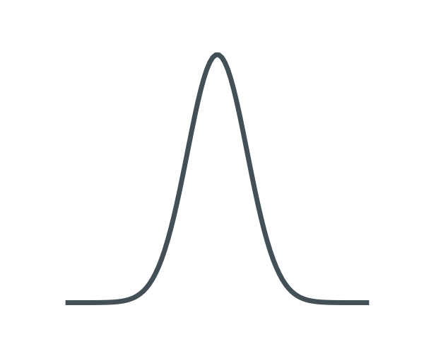
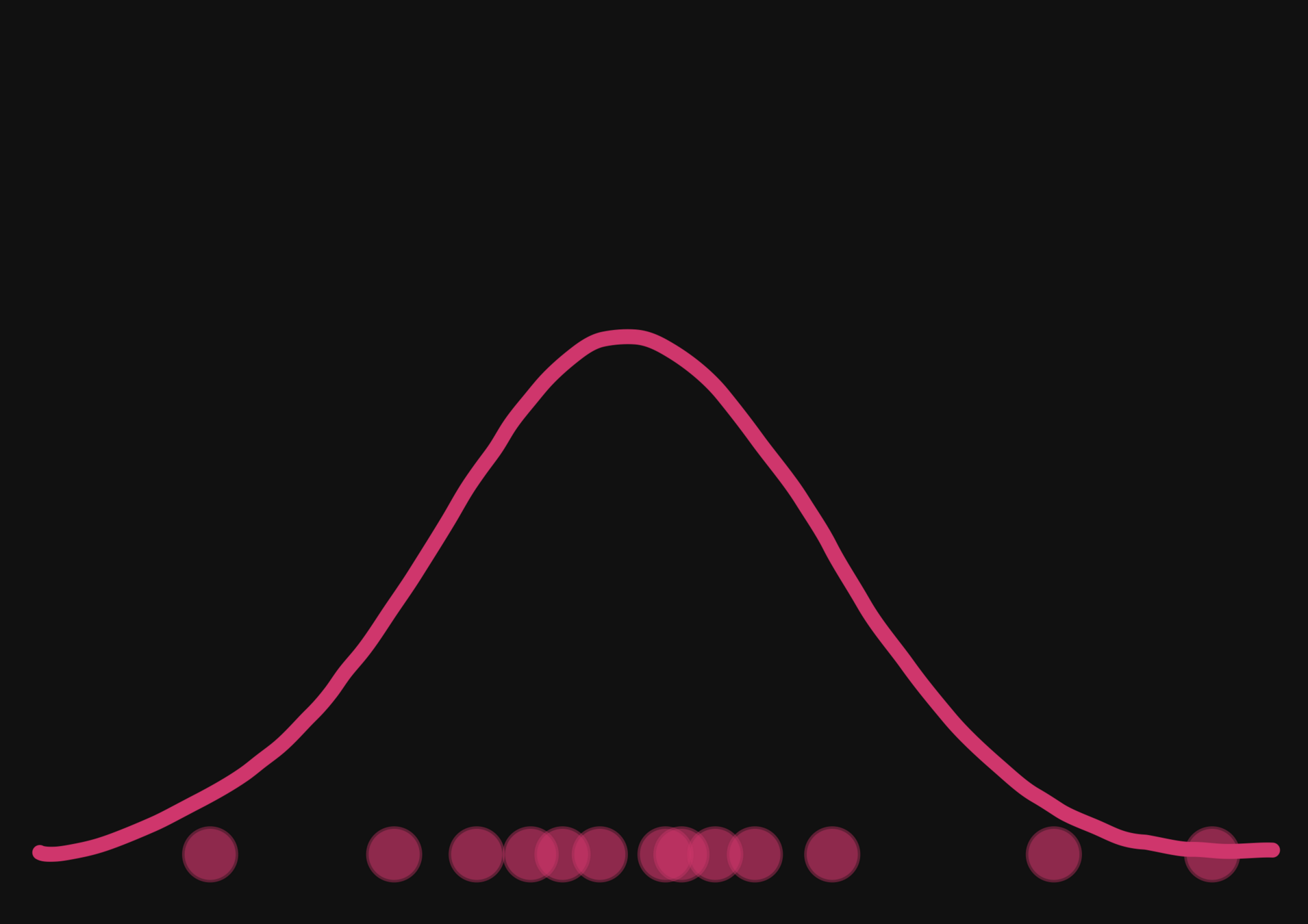
\text{True distribution } p(x)
\text{Sample } x \sim p(x)
\text{Model } p_{\phi}(x)

We need a model that can approximate distributions from its samples.
Easy to evaluate
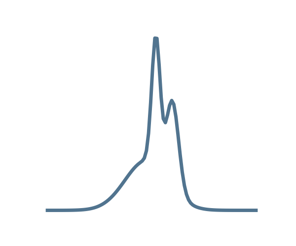
Neural Density Estimator
We need a model that can approximate distributions from its samples.
\text{True distribution } p(x)
\text{Sample } x \sim p(x)
\text{Model } p_{\phi}(x)

Easy to evaluate
and sample
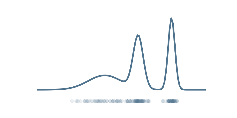
Neural Density Estimator
We need a model that can approximate distributions from its samples.
\text{True distribution } p(x)
\text{Sample } x \sim p(x)
\text{Model } p_{\phi}(x)
Easy to evaluate
and sample
Normalizing Flows
Normalizing Flows
reference: https://blog.evjang.com/2019/07/nf-jax.html
Normalizing Flows
p_x(x)
p_z(z)
f(z)
\text{sampling}
Normalizing Flows
p_x(x)
p_z(z)
Normalizing Flows
p_x(x)
p_z(z)
Normalizing Flows
p_x(x)
p_z(z)
Normalizing Flows
p_x(x)
p_z(z)
f^{-1}(x)
\text{evaluation}
Normalizing Flows
p_x(x)
p_z(z)
f^{-1}(x)
\text{evaluation}
\log p_x(x) = \log p_z(f^{-1}(x))
Normalizing Flows
p_x(x)
p_z(z)
f^{-1}(x)
\text{evaluation}
\log p_x(x) = \log p_z(f^{-1}(x))
+ \log
\displaystyle\left\lvert det \frac{\partial f^{-1}(x)}{\partial x}\right\rvert
Change of Variable Formula:
Normalizing Flows
p_x(x)
p_z(z)
f^{-1}(x)
\text{evaluation}
f(z)
\text{sampling}
\log p_x(x) = \log p_z(f^{-1}(x))
+ \log
\displaystyle\left\lvert det \frac{\partial f^{-1}(x)}{\partial x}\right\rvert
Change of Variable Formula:
Normalizing Flows
p_x(x)
p_z(z)
f^{-1}(x)
\text{evaluation}
f(z)
\text{sampling}
We need to learn the mapping
to approximate the complex distribution.
Normalizing Flows
p_x(x)
p_z(z)
f^{-1}(x)
\text{evaluation}
f(z)
\text{sampling}
p_x(x)
True distribution
We need to learn the mapping
to approximate the complex distribution.
Normalizing Flows
p_x(x)
p_z(z)
g^{-1}(x)
\text{evaluation}
g(z)
\text{sampling}
p_x(x)
True distribution
It seems to be the one!
How to train a Normalizing Flow?
\text{ $\to$ we need a tool to compare distributions:}\\
\textbf{the Kullback-Leiber Divergence}
How to train a Normalizing Flow?
\begin{array}{ll}
D_{KL}(p_x(x)||p_x^{\phi}(x)) &= \mathbb{E}_{p_x(x)}\Big[ \log\left(\frac{p_x(x)}{p_x^{\phi}(x)}\right) \Big] \\
\end{array}
\begin{array}{ll}
= \mathbb{E}_{p_x(x)}\left[ \log\left(p_x(x)\right) \right]
\end{array}
\begin{array}{ll}
- \mathbb{E}_{p_x(x)}\left[ \log\left(p_x^{\phi}(x)\right) \right]\\
\end{array}
\begin{array}{ll}
= \mathbb{E}_{p_x(x)}\left[ \log\left(p_x(x)\right) \right]
\end{array}
\begin{array}{ll}
- \mathbb{E}_{p_x(x)}\left[ \log\left(p_x^{\phi}(x)\right) \right]\\
\end{array}
Variational parameters related to the mapping
How to train a Normalizing Flow?
\begin{array}{ll}
D_{KL}(p_x(x)||p_x^{\phi}(x)) &= \mathbb{E}_{p_x(x)}\Big[ \log\left(\frac{p_x(x)}{p_x^{\phi}(x)}\right) \Big] \\
\end{array}
\begin{array}{ll}
= \mathbb{E}_{p_x(x)}\left[ \log\left(p_x(x)\right) \right]
\end{array}
\begin{array}{ll}
- \mathbb{E}_{p_x(x)}\left[ \log\left(p_x^{\phi}(x)\right) \right]\\
\end{array}
\begin{array}{ll}
= \mathbb{E}_{p_x(x)}\left[ \log\left(p_x(x)\right) \right]
\end{array}
\begin{array}{ll}
- \mathbb{E}_{p_x(x)}\left[ \log\left(p_x^{\phi}(x)\right) \right]\\
\end{array}
\text{
We want to minimize the Kullback-Leiber Divergence wrt $\phi$
}
How to train a Normalizing Flow?
\begin{array}{ll}
D_{KL}(p_x(x)||p_x^{\phi}(x)) &= \mathbb{E}_{p_x(x)}\Big[ \log\left(\frac{p_x(x)}{p_x^{\phi}(x)}\right) \Big] \\
\end{array}
\begin{array}{ll}
= \mathbb{E}_{p_x(x)}\left[ \log\left(p_x(x)\right) \right]
\end{array}
\begin{array}{ll}
- \mathbb{E}_{p_x(x)}\left[ \log\left(p_x^{\phi}(x)\right) \right]\\
\end{array}
\begin{array}{ll}
\mathbb{E}_{p_x(x)}\left[ \log\left(p_x(x)\right) \right]
\end{array}
\begin{array}{ll}
- \mathbb{E}_{p_x(x)}\left[ \log\left(p_x^{\phi}(x)\right) \right]\\
\end{array}
\text{
We want to minimize the Kullback-Leiber Divergence wrt $\phi$
}
How to train a Normalizing Flow?
\begin{array}{ll}
D_{KL}(p_x(x)||p_x^{\phi}(x)) &= \mathbb{E}_{p_x(x)}\Big[ \log\left(\frac{p_x(x)}{p_x^{\phi}(x)}\right) \Big] \\
\end{array}
\begin{array}{ll}
= \mathbb{E}_{p_x(x)}\left[ \log\left(p_x(x)\right) \right]
\end{array}
\begin{array}{ll}
- \mathbb{E}_{p_x(x)}\left[ \log\left(p_x^{\phi}(x)\right) \right]\\
\end{array}
\text{constant}
\begin{array}{ll}
- \mathbb{E}_{p_x(x)}\left[ \log\left(p_x^{\phi}(x)\right) \right]\\
\end{array}
\text{
We want to minimize the Kullback-Leiber Divergence wrt $\phi$
}
How to train a Normalizing Flow?
\begin{array}{ll}
D_{KL}(p_x(x)||p_x^{\phi}(x)) &= \mathbb{E}_{p_x(x)}\Big[ \log\left(\frac{p_x(x)}{p_x^{\phi}(x)}\right) \Big] \\
\end{array}
\begin{array}{ll}
= \mathbb{E}_{p_x(x)}\left[ \log\left(p_x(x)\right) \right]
\end{array}
\begin{array}{ll}
- \mathbb{E}_{p_x(x)}\left[ \log\left(p_x^{\phi}(x)\right) \right]\\
\end{array}
\text{
We want to minimize the Kullback-Leiber Divergence wrt $\phi$
}
\begin{array}{ll}
\implies Loss = - \mathbb{E}_{x \sim p_x(x)}\left[ \log\left(p_x^{\phi}(x)\right) \right]\\
\end{array}
\text{constant}
\begin{array}{ll}
- \mathbb{E}_{p_x(x)}\left[ \log\left(p_x^{\phi}(x)\right) \right]\\
\end{array}
How to train a Normalizing Flow?
\begin{array}{ll}
D_{KL}(p_x(x)||p_x^{\phi}(x)) &= \mathbb{E}_{p_x(x)}\Big[ \log\left(\frac{p_x(x)}{p_x^{\phi}(x)}\right) \Big] \\
\end{array}
\begin{array}{ll}
= \mathbb{E}_{p_x(x)}\left[ \log\left(p_x(x)\right) \right]
\end{array}
\begin{array}{ll}
- \mathbb{E}_{p_x(x)}\left[ \log\left(p_x^{\phi}(x)\right) \right]\\
\end{array}
\text{
We want to minimize the Kullback-Leiber Divergence wrt $\phi$
}
From simulations of the true distribution only!
\begin{array}{ll}
\implies Loss = - \mathbb{E}_{x \sim p_x(x)}\left[ \log\left(p_x^{\phi}(x)\right) \right]\\
\end{array}
\text{constant}
\begin{array}{ll}
- \mathbb{E}_{p_x(x)}\left[ \log\left(p_x^{\phi}(x)\right) \right]\\
\end{array}
Normalizing Flows for Implicit Inference
\begin{array}{ll}
Loss_{NLE} = - \mathbb{E}_{p(x, \theta)}\left[ \log\left(p_{\phi}(x\:|\:\theta)\right) \right]\\
\end{array}
\text{Similarly for NLE or NPE we can train the NF to approximate } p(x\:|\:\theta)
\text{ or } p(\theta\:|\:x) \\ \text{ from samples } (\theta_i, x_i)_{i=1...N} \sim p(x, \theta)
\begin{array}{ll}
Loss_{NPE} = - \mathbb{E}_{p(x, \theta)}\left[ \log\left(p_{\phi}(\theta\:|\:x)\right) \right]\\
\end{array}
This is super nice, it allows us to approximate the posterior distribution from simulations ONLY!
But simulations can sometimes be very expensive and training a NF requires a lot of simulations..
Neural Posterior Estimation with Differentiable Simulators
ICML 2022 Workshop on Machine Learning for Astrophysics
Justine Zeghal, François Lanusse, Alexandre Boucaud,
Benjamin Remy and Eric Aubourg
x
\theta
z
f
\sigma^2
\mathcal{N}
Explicit joint likelihood
p(x| \theta, z)
p(x| \theta, z)
\nabla_{\theta} \log p(\theta, z |x) =
x
\theta
z
f
\sigma^2
\mathcal{N}
Explicit joint likelihood
p(x| \theta, z)
p(x| \theta, z)
\nabla_{\theta} \log p(x| \theta, z)
\nabla_{\theta} \log p(\theta, z |x) =
x
\theta
z
f
\sigma^2
\mathcal{N}
Explicit joint likelihood
p(x| \theta, z)
p(x| \theta, z)
+ \nabla_{\theta} \log p(\theta)
+ \nabla_{\theta} \log p(z|\theta)
\nabla_{\theta} \log p(x| \theta, z)
\nabla_{\theta} \log p(\theta, z |x) =
x
\theta
f
\sigma^2
\mathcal{N}
Explicit joint likelihood
p(x| \theta, z)
p(x| \theta, z)
z
+ \nabla_{\theta} \log p(\theta)
+ \nabla_{\theta} \log p(z|\theta)
\nabla_{\theta} \log p(x| \theta, z)
\nabla_{\theta} \log p(\theta, z |x) =

a framework for automatic differentiation following the NumPy API, and using GPU
probabilistic programming library
powered by JAX
x
\theta
z
f
\sigma^2
\mathcal{N}
Explicit joint likelihood
p(x| \theta, z)
p(x| \theta, z)


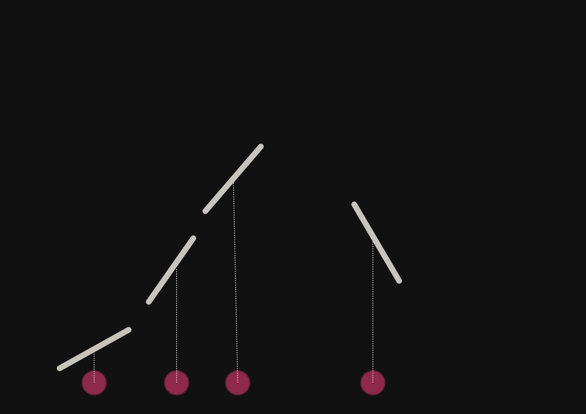
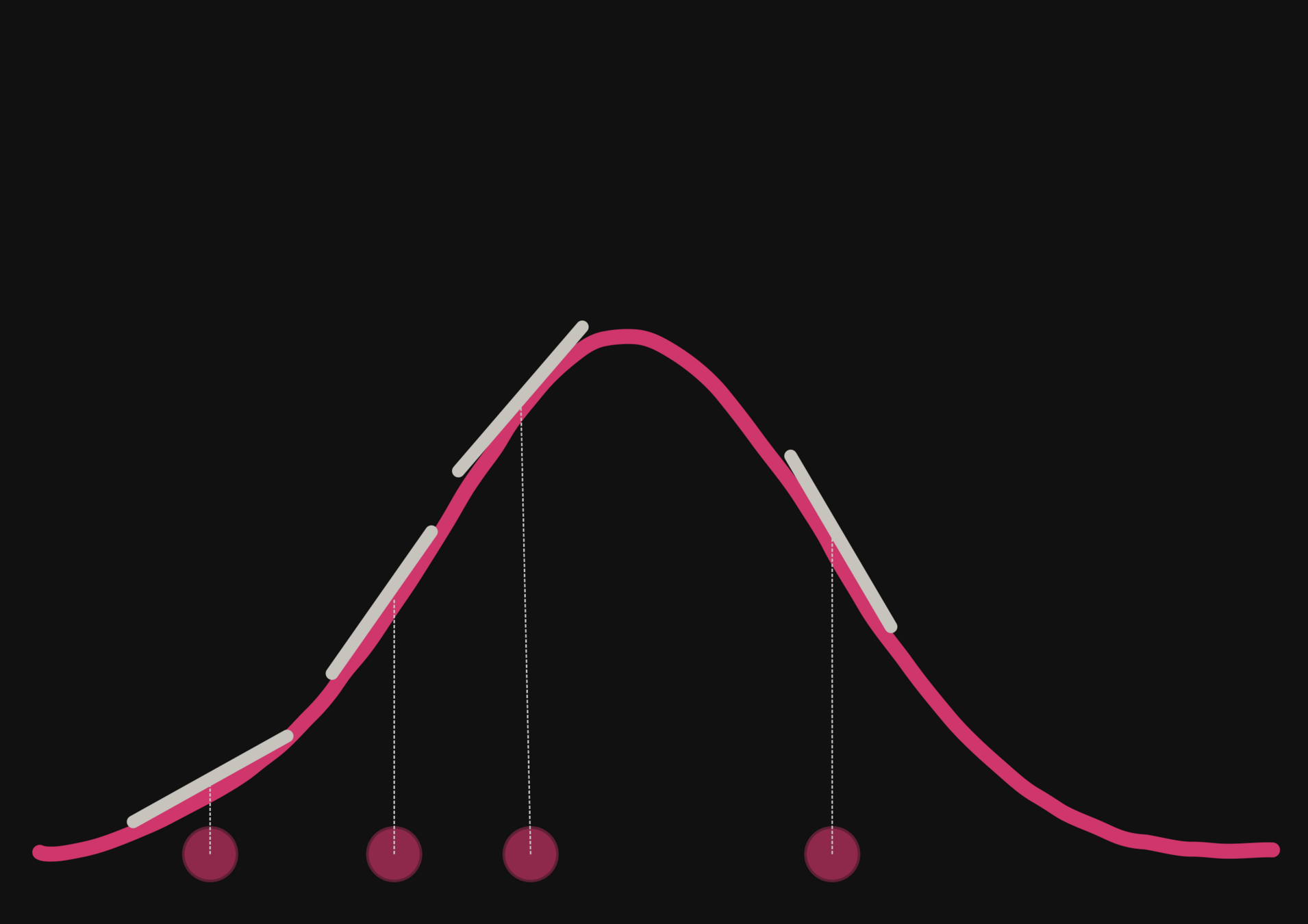
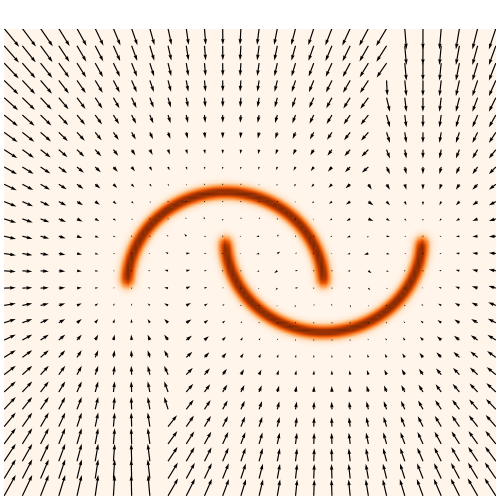
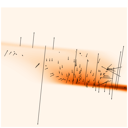
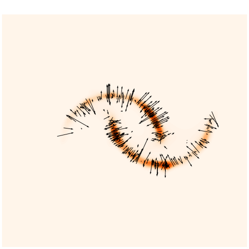
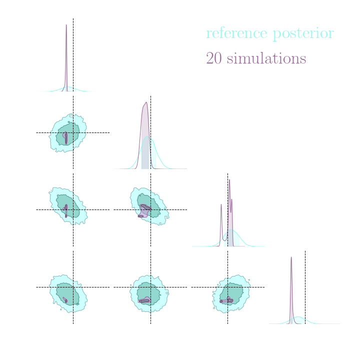
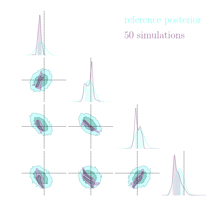
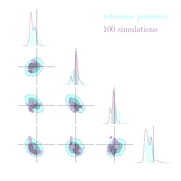
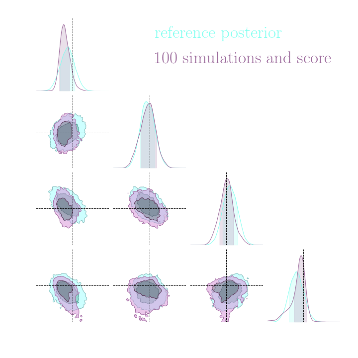
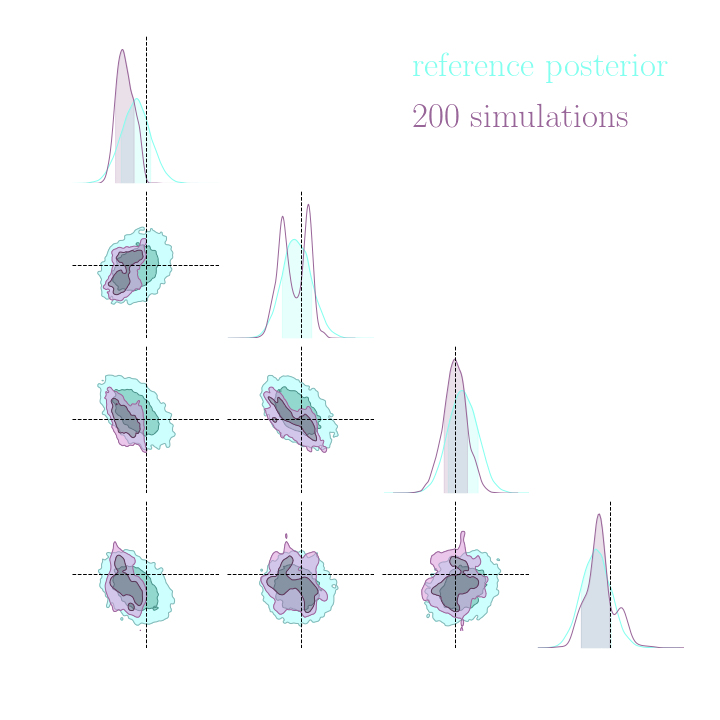
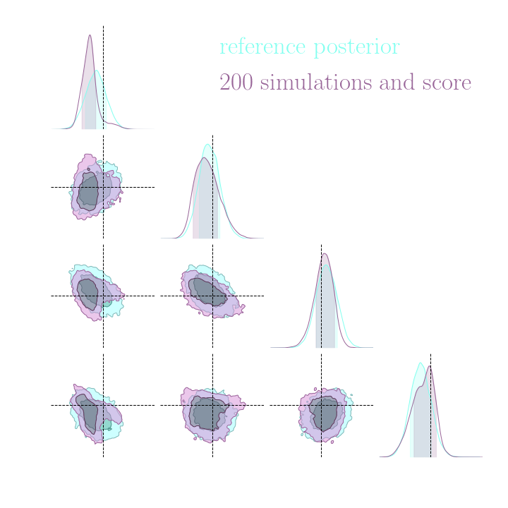
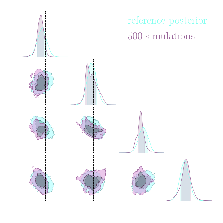
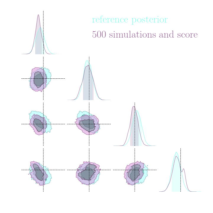
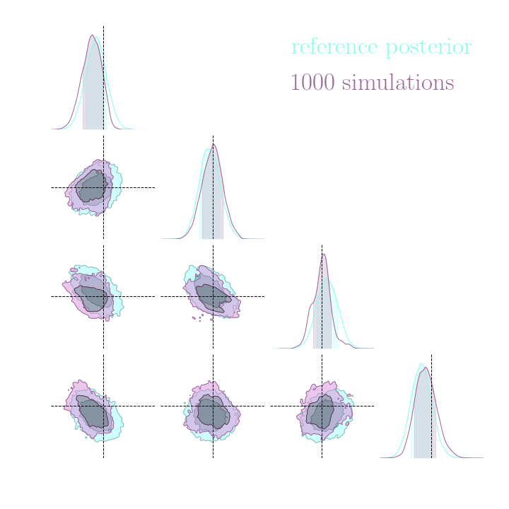
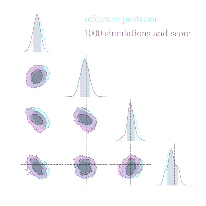
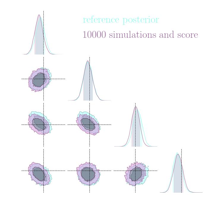
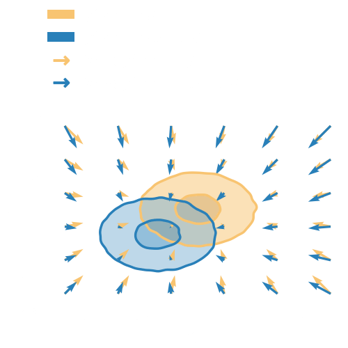
With a few simulations it's hard to approximate the posterior distribution.
→ we need more simulations
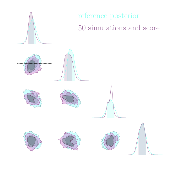
BUT if we have a few simulations
and the gradients
(also know as the score)
\nabla_{\theta} \log p(\theta | x)
then it's possible to have an idea of the shape of the distribution.
How gradients can help Implicit Inference?
How to train NFs with gradients?
How to train NFs with gradients?
Normalizing flows are trained by minimizing the negative log likelihood:
- \mathbb{E}_{p(x, \theta)}\left[ \log\left(p^{\phi}(\theta | x)\right) \right]
How to train NFs with gradients?
But to train the NF, we want to use both simulations and gradient
- \mathbb{E}_{p(x, \theta)}\left[ \log\left(p^{\phi}(\theta | x)\right) \right]
Normalizing flows are trained by minimizing the negative log likelihood:
- \mathbb{E}_{p(x, \theta)}\left[ \log\left(p^{\phi}(\theta | x)\right) \right]
How to train NFs with gradients?
+ \: \lambda \: \displaystyle \mathbb{E}\left[ \parallel \nabla_{\theta} \log p(\theta, z |x) - \nabla_{\theta} \log p^{\phi}(\theta |x)\parallel_2^2 \right]
- \mathbb{E}_{p(x, \theta)}\left[ \log\left(p^{\phi}(\theta | x)\right) \right]
But to train the NF, we want to use both simulations and gradient
Normalizing flows are trained by minimizing the negative log likelihood:
- \mathbb{E}_{p(x, \theta)}\left[ \log\left(p^{\phi}(\theta | x)\right) \right]
How to train NFs with gradients?
- \mathbb{E}_{p(x, \theta)}\left[ \log\left(p^{\phi}(\theta | x)\right) \right]
But to train the NF, we want to use both simulations and gradient
Normalizing flows are trained by minimizing the negative log likelihood:
- \mathbb{E}_{p(x, \theta)}\left[ \log\left(p^{\phi}(\theta | x)\right) \right]
+ \: \lambda \: \displaystyle \mathbb{E}\left[ \parallel \nabla_{\theta} \log p(\theta, z |x) - \nabla_{\theta} \log p^{\phi}(\theta |x)\parallel_2^2 \right]
How to train NFs with gradients?
Problem: the gradient of current NFs lack expressivity
- \mathbb{E}_{p(x, \theta)}\left[ \log\left(p^{\phi}(\theta | x)\right) \right]
But to train the NF, we want to use both simulations and gradient
Normalizing flows are trained by minimizing the negative log likelihood:
- \mathbb{E}_{p(x, \theta)}\left[ \log\left(p^{\phi}(\theta | x)\right) \right]
+ \: \lambda \: \displaystyle \mathbb{E}\left[ \parallel \nabla_{\theta} \log p(\theta, z |x) - \nabla_{\theta} \log p^{\phi}(\theta |x)\parallel_2^2 \right]
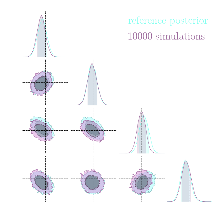
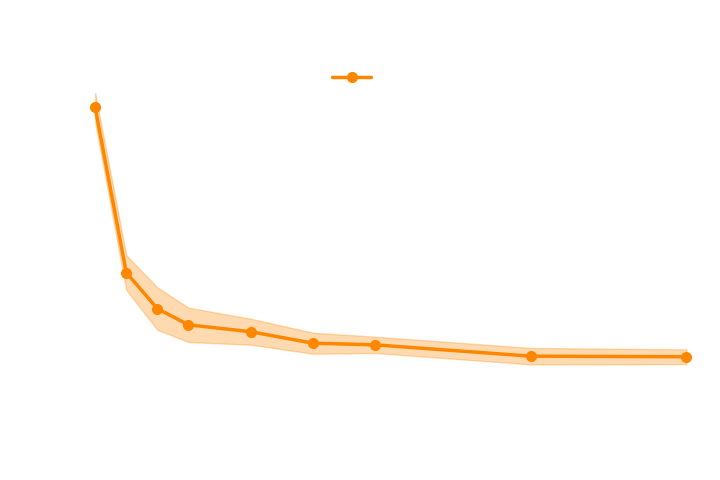
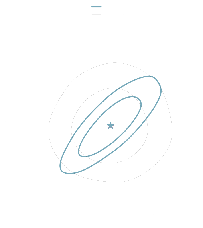
Results on a toy model


→ On a toy Lotka Volterra model, the gradients helps to constrain the distribution shape.
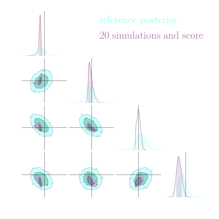
Results on a toy model
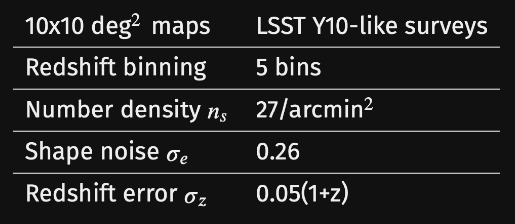
Simulation-Based Inference Benchmark for LSST Weak Lensing Cosmology
Justine Zeghal, Denise Lanzieri, François Lanusse, Alexandre Boucaud, Gilles Louppe, Eric Aubourg,
and The LSST Dark Energy Science Collaboration (LSST DESC)
-
do gradients help implicit inference methods?
In the case of weak lensing full-field analysis,
-
which inference method requires the fewest simulations?
x
\theta
z
f
\sigma^2
\mathcal{N}
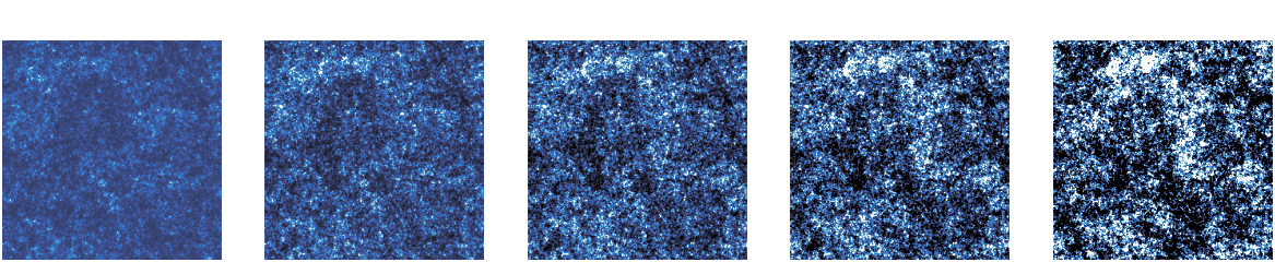
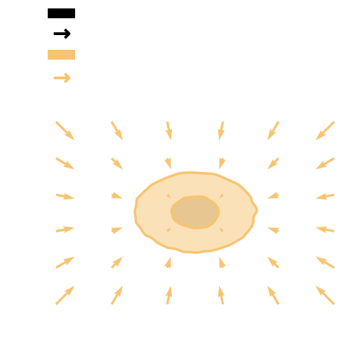
We developed a fast and differentiable (JAX) log-normal mass maps simulator
For our benchmark: a Differentiable Mass Maps Simulator

-
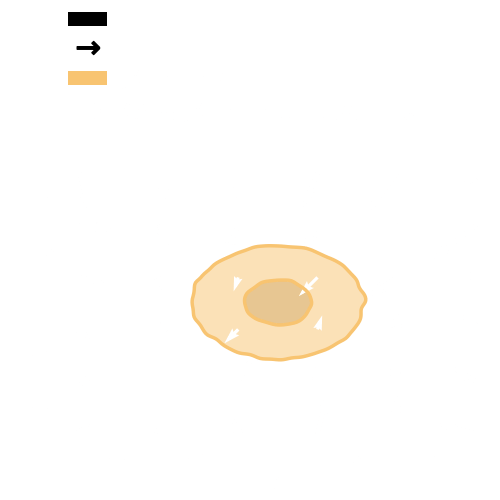
Do gradients help implicit inference methods?
- \mathbb{E}_{p(x, \theta)}\left[ \log\left(p^{\phi}(x | \theta)\right) \right]
+ \: \lambda \: \displaystyle \mathbb{E}\left[ \parallel \nabla_{\theta} \log p(x, z |\theta) -{\nabla_{\theta} \log p^{\phi}(x|\theta )}\parallel_2^2 \right]
Training the NF with simulations and gradients:
Loss =
-
Do gradients help implicit inference methods?
- \mathbb{E}_{p(x, \theta)}\left[ \log\left(p^{\phi}(x | \theta)\right) \right]
+ \: \lambda \: \displaystyle \mathbb{E}\left[ \parallel \nabla_{\theta} \log \hat{p}(x |\theta) -{\nabla_{\theta} \log p^{\phi}(x|\theta )}\parallel_2^2 \right]
Training the NF with simulations and gradients:
Loss =
-
Do gradients help implicit inference methods?
\nabla_{\theta}\log p(x|\theta)
\nabla_{\theta}\log p(x,z|\theta)
(from the simulator)
(requires a lot of additional simulations)
→ For this particular problem, the gradients from the simulator are too noisy to help.
-
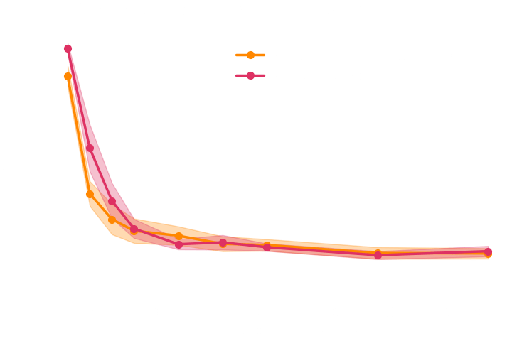
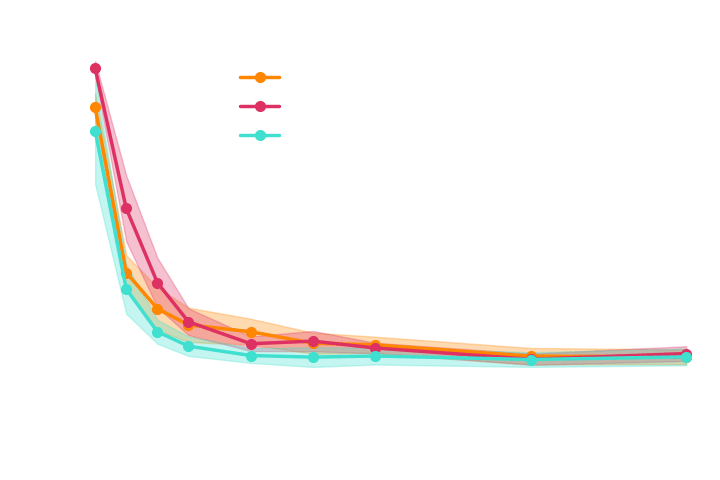
Do gradients help implicit inference methods?
→ Implicit inference (NLE) requires 1500 simulations.
→ Better to use NLE without gradients than NLE with gradients.
-
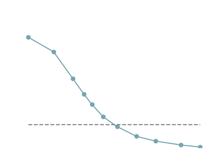
Which inference method requires the fewest simulations?
→ Implicit inference (NLE) requires 1500 simulations.
→ What about explicit inference?
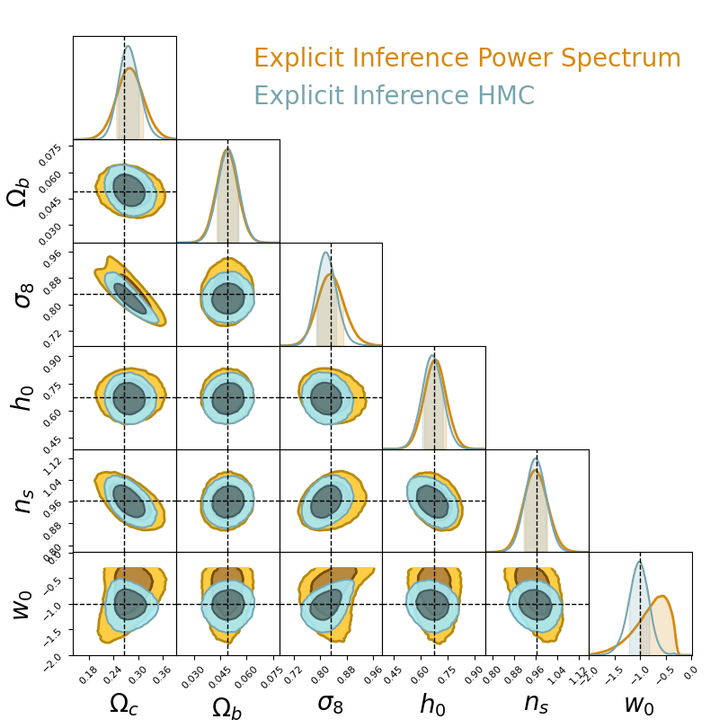
→ Explicit inference requires 10^5 simulations.
simulations
simulations
10^5
10 ^ 3
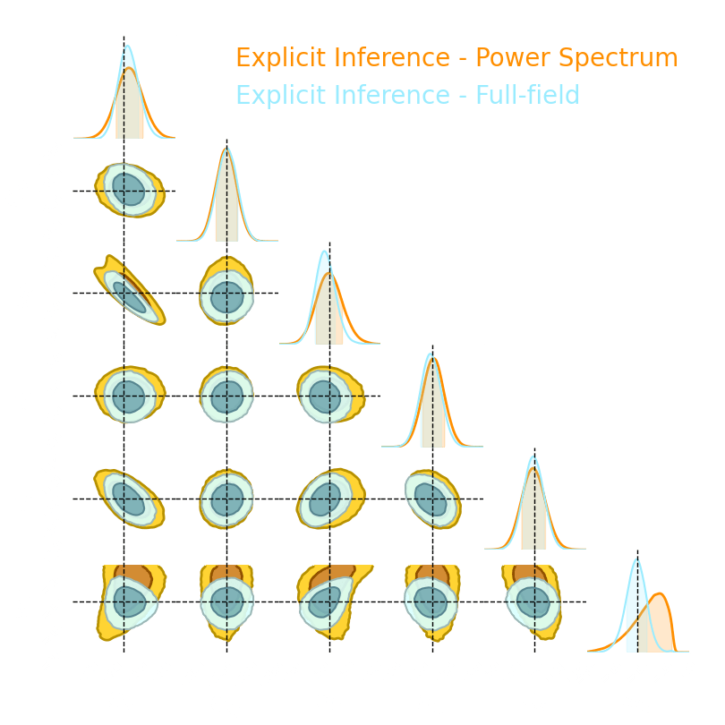
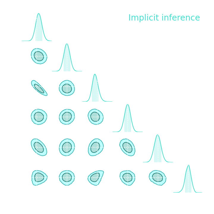
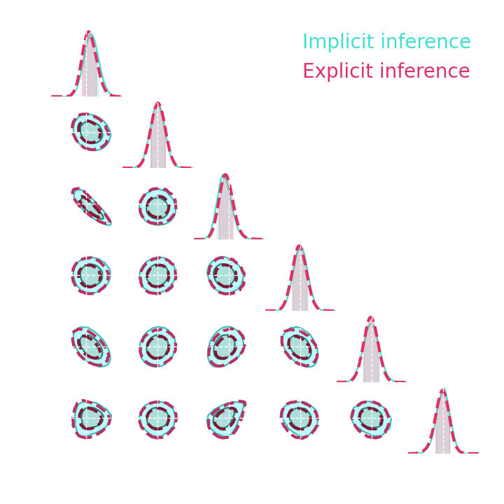
→ Explicit and implicit full-field inference yields the same posterior.
→ Explicit full-field inference requires 630 000 simulations (HMC in high dimension)
→ Implicit full-field inference requires 1 500 simulations
+ a maximum of 100 000 simulations to build
sufficient statistics
-
Which inference method requires the fewest simulations?
Optimal Neural Summarisation for Full-Field Weak Lensing Cosmological Implicit Inference
Denise Lanzieri, Justine Zeghal, T. Lucas Makinen, François Lanusse, Alexandre Boucaud and Jean-Luc Starck
\theta
Summary statistics
t = f_{\varphi}(x)
x
p_{\Phi}(\theta | f_{\varphi}(x))
Simulator
Summary statistics
t = f_{\varphi}(x)
x
p_{\Phi}(\theta | f_{\varphi}(x))
\theta
Simulator
Summary statistics
t = f_{\varphi}(x)
x
p_{\Phi}(\theta | f_{\varphi}(x))
\theta
Simulator
x

t = f_{\varphi}(x)
\text{A statistic } t \text{ is said to be sufficient for the parameters } \theta \text{ if }
\text{Sufficient statistic}
p(\theta \: | \: x) = p(\theta \: | \: t) \: \text{ with } \: t=f(x)
How to extract all the information?
It is only a matter of the loss function you use to train your compressor..
Two ways..
1) Regression
\hat{\theta} = f(x)
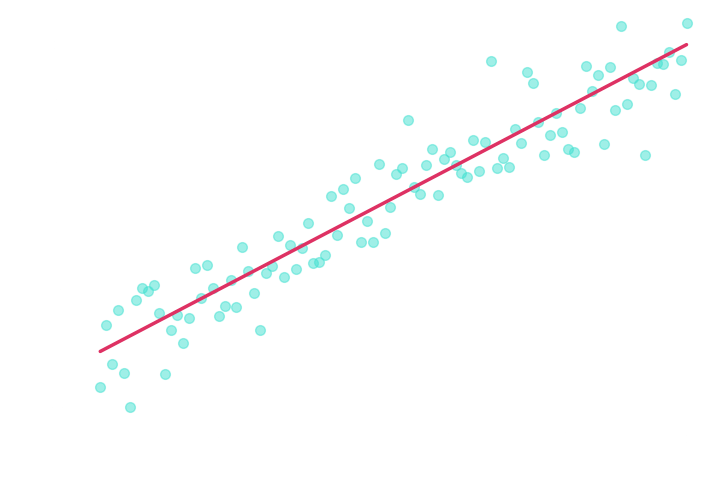
\hat{\theta} = f(x)
Which learns a moment of the posterior distribution and is not guaranteed to be sufficient.
Two ways..
1) Regression
\hat{\theta} = f(x)
Which learns a moment of the posterior distribution and is not guaranteed to be sufficient.
Two ways..
1) Regression
\hat{\theta} = f(x)
Which learns a moment of the posterior distribution and is not guaranteed to be sufficient.
Two ways..
1) Regression
\mu_1 = \mu_2
\hat{\theta} = f(x)
Which learns a moment of the posterior distribution and is not guaranteed to be sufficient.
Two ways..
1) Regression
\mu_1 = \mu_2
\hat{\theta} = f(x)
Which learns a moment of the posterior distribution and is not guaranteed to be sufficient.
Two ways..
1) Regression
\mu_1 = \mu_2
\hat{\theta} = f(x)
Which learns a moment of the posterior distribution and is not guaranteed to be sufficient.
Two ways..
1) Regression
\neq
Not a sufficient statistics
\hat{\theta} = f(x)
Which learns a moment of the posterior distribution and is not guaranteed to be sufficient.
Two ways..
1) Regression
Two ways..
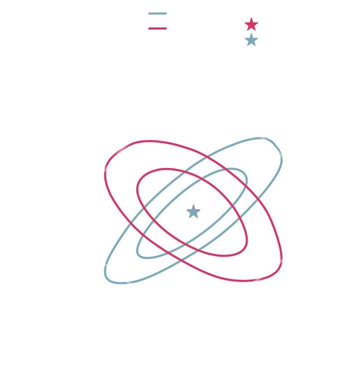
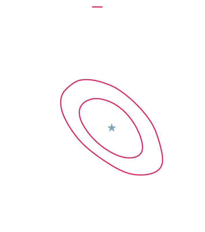
2) Mutual information maximization
p(\theta \: | \: x) = p(\theta \: | \: t(x)) \: \Leftrightarrow I(\theta, x) = I (\theta, t(x))
I(\theta,t)
H(\theta)
H(t)
H(\theta|t)
H(t|\theta)
I(\theta,t) = H(t) - H(t|\theta)
Two ways..
2) Mutual information maximization
p(\theta \: | \: x) = p(\theta \: | \: t(x)) \: \Leftrightarrow I(\theta, x) = I (\theta, t(x))
I(\theta,t)
H(\theta)
H(t)
H(\theta|t)
H(t|\theta)
I(\theta,t) = H(t) - H(t|\theta)
Two ways..
2) Mutual information maximization
p(\theta \: | \: x) = p(\theta \: | \: t(x)) \: \Leftrightarrow I(\theta, x) = I (\theta, t(x))
I(\theta,x)
I(\theta,t) = H(t) - H(t|\theta)
Two ways..
2) Mutual information maximization
p(\theta \: | \: x) = p(\theta \: | \: t(x)) \: \Leftrightarrow I(\theta, x) = I (\theta, t(x))
I(\theta,t) = H(t) - H(t|\theta)
Two ways..
2) Mutual information maximization
p(\theta \: | \: x) = p(\theta \: | \: t(x)) \: \Leftrightarrow I(\theta, x) = I (\theta, t(x))
I(\theta,t) = H(t) - H(t|\theta)
Two ways..
p(\theta \: | \: x) = p(\theta \: | \: t(x)) \: \Leftrightarrow I(\theta, x) = I (\theta, t(x))
2) Mutual information maximization
I(\theta,t) = H(t) - H(t|\theta)
Two ways..
p(\theta \: | \: x) = p(\theta \: | \: t(x)) \: \Leftrightarrow I(\theta, x) = I (\theta, t(x))
2) Mutual information maximization
→ should build sufficient statistics
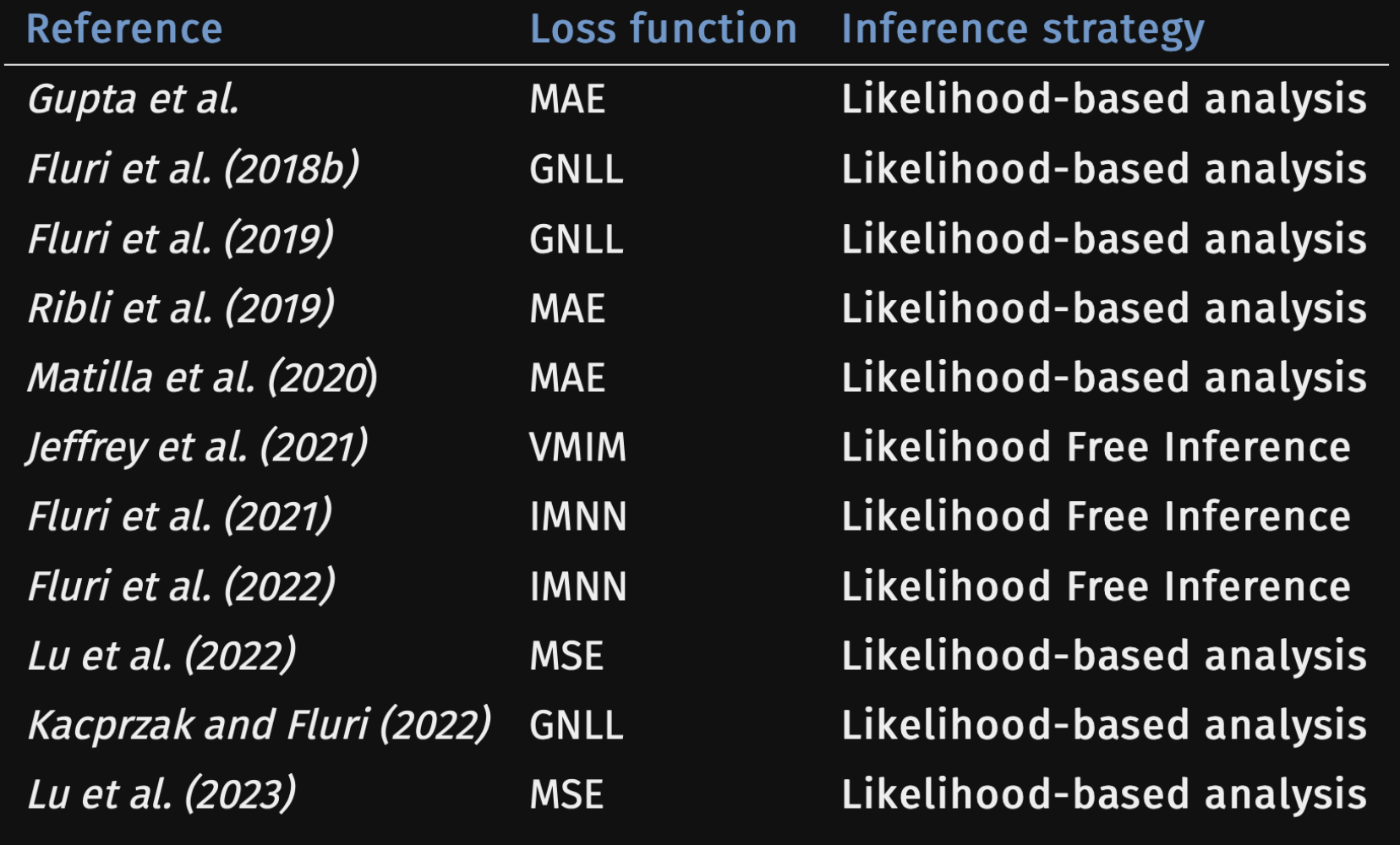
For our benchmark
Log-normal LSST Y10 like
differentiable
simulator

t = f_{\varphi}(x)

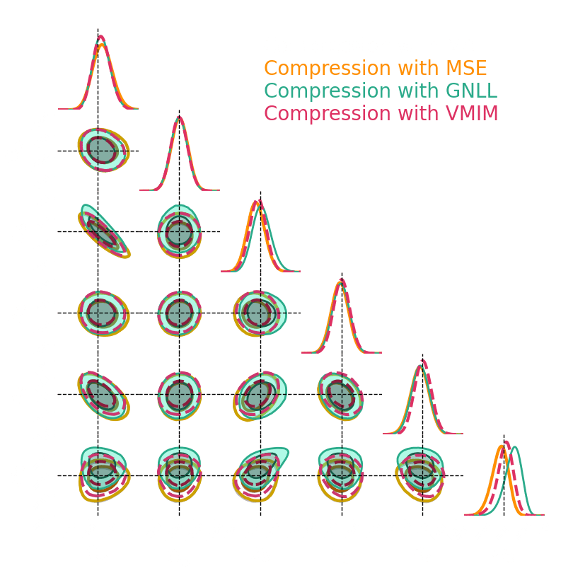
1. We compress using one of the 4 losses.
Benchmark procedure:
2. We compare their extraction power by comparing their posteriors.
For this, we use a neural-based likelihood-free approach, which is fixed for all the compression strategies.
p(\theta \: | \: x) = p(\theta \: | \: t) \: \text{ with } \: t=f(x)
Numerical results
compression schemes based on regression losses are not guaranteed to build such sufficient statistics
Takeaways
Compression schemes based on information maximization can build sufficient statistics
while
Summary
\underbrace{p(\theta|x=x_0)}_{\text{posterior}}
\underbrace{p(\theta)}_{\text{prior}}
\underbrace{p(x = x_0|\theta)}_{\text{likelihood}}
\propto
Summary
\underbrace{p(\theta|x=x_0)}_{\text{posterior}}
\underbrace{p(\theta)}_{\text{prior}}
\underbrace{p(x = x_0|\theta)}_{\text{likelihood}}
\propto
x
\theta
z
f
\sigma^2
\mathcal{N}
Explicit likelihood
Summary
\underbrace{p(\theta|x=x_0)}_{\text{posterior}}
\underbrace{p(\theta)}_{\text{prior}}
\underbrace{p(x = x_0|\theta)}_{\text{likelihood}}
\propto
x
\theta
z
f
\sigma^2
\mathcal{N}
Explicit likelihood
x
\theta
z
f
Simulator
Implicit likelihood
Summary
\underbrace{p(\theta|x=x_0)}_{\text{posterior}}
\underbrace{p(\theta)}_{\text{prior}}
\underbrace{p(x = x_0|\theta)}_{\text{likelihood}}
\propto
Explicit likelihood
Implicit likelihood
x
\theta
f
Simulator
Explicit inference
or
Implicit inference
Summary
\underbrace{p(\theta|x=x_0)}_{\text{posterior}}
\underbrace{p(\theta)}_{\text{prior}}
\underbrace{p(x = x_0|\theta)}_{\text{likelihood}}
\propto
Explicit likelihood
Implicit likelihood
Implicit inference
Explicit inference
or
Implicit inference
Summary
Implicit inference
Explicit inference
Summary
Implicit inference
Explicit inference
- MCMC in high-dimension
- Challenging to sample
- Needs the gradients
- simulations (on our problem)
10^5
Summary
Implicit inference
Explicit inference
- MCMC in high-dimension
- Challenging to sample
- Needs the gradients
- simulations (on our problem)
10^5
10 ^ 3
- Based on machine learning
- Only need simulations
- Gradients can be used but do not help in our problem
- simulations (on our problem)
- Better to do one compression step before (Mutual information maximization)
Summary
Implicit inference
Explicit inference
- MCMC in high-dimension
- Challenging to sample
- Needs the gradients
- simulations (on our problem)
10^5
- Based on machine learning
- Only need simulations
- Gradients can be used but do not help in our problem
- simulations (on our problem)
- Better to do one compression step before (Mutual information maximization)
10 ^ 3
\theta
f
\mathcal{N}
Simulator
Summary statistics
t = f_{\varphi}(x)
x
p_{\Phi}(\theta | f_{\varphi}(x))
Thank you for your attention!
Rencontres Statistiques Lyonnaises
By Justine Zgh


