行動技術與應用
Lesson 9: Convolutional Neural Network
Outline
- Keras R安裝與運作回顧
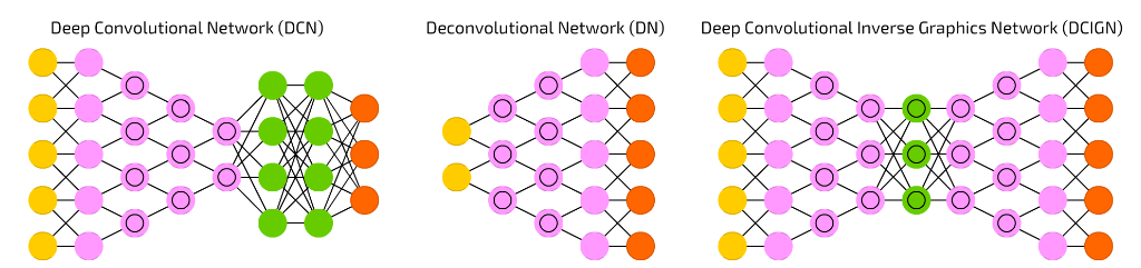
- 什麼是「卷積神經網路」(CNN)
- 卷積神經網路應用於MNIST資料集
Keras R安裝回顧
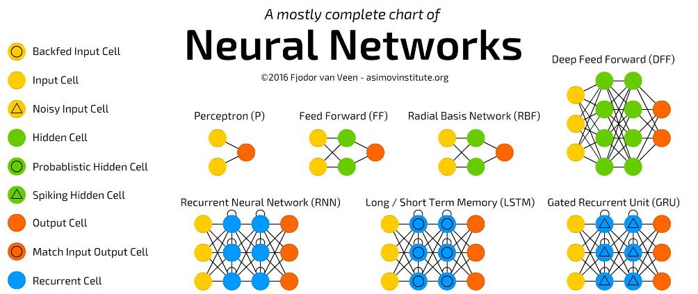
NN圖解

輸入層
隱藏層
卷積核
TensorFlow/Keras(R版本)安裝
R-Keras開發環境: 總整理

r-tensorflow

conda create --name r-tensorflow python=3.7
activate r-tensorflow
pip install -I -U tensorflow
conda install -c conda-forge keras


(R Rtools)

TensorFlow R
keras R
devtools::install_github("rstudio/tensorflow")
devtools::install_github("rstudio/keras")

library(keras)   ## Keras for R

❹
❶
❷
❸
❺
TensorFlow/Keras(R版本) 測試1
在RStudio內測試rstudio/tensorflow
```{r eval=FALSE}
# 安裝'devtools' package:方便從github安裝套件
if(!"devtools" %in% installed.packages())
  install.packages('devtools')

require(devtools)

# install tensorflow(如果你要tensorflow的話)
devtools::install_github("rstudio/tensorflow")

# installing keras(如果你要keras的話)
devtools::install_github("rstudio/keras")
```

```{r eval=FALSE}
# 測試tensorflow: Hello
require(tensorflow)
session = tf$Session()
hello <- tf$constant('Hi, TensorFlow!')
session$run(hello)
```
hello.rmd
TensorFlow/Keras(R版本) 測試2
在RStudio內測試rstudio/keras
```{r eval=FALSE}
library(keras)
model <- keras_model_sequential()
model %>%
layer_dense(units = 256, activation = 'relu', input_shape= c(784)) %>%
layer_dropout(rate = 0.4) %>%
layer_dense(units = 128, activation = 'relu') %>%
layer_dropout(rate = 0.3) %>%
layer_dense(units = 10, activation = 'softmax')
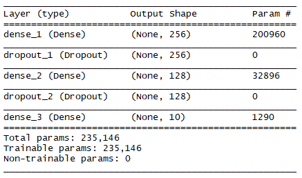
summary(model)
```keras.rmd
Keras 基本運作方式回顧
- 安裝keras R
- 準備資料集: 訓練集/測試集- 以FashionMinst資料集為例
- 建立深度學習模型: Sequential Model
- 建立模型: 隱藏層
- 編譯模型: 損失函數、優化演算法
- 訓練與評估(模型正確機率)
- 目的: 找出最適函數(最佳預測函數)
- 應用(預測)
Keras R安裝Keras R套件
- 安裝 Keras R套件
```{r eval=FALSE}
if(!"devtools" %in% installed.packages())
  install.packages("devtools");

if(!"keras" %in% installed.packages()) {
  require(devtools);
  install_github("rstudio/keras");
}

library(keras)
install_keras()  # 如需GPU設定,參考文件網址
```
install_keras() 文件網址:https://keras.rstudio.com/reference/install_keras.html
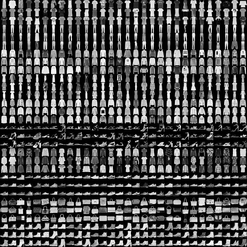
Keras R準備資料: Fashion-MNIST資料集
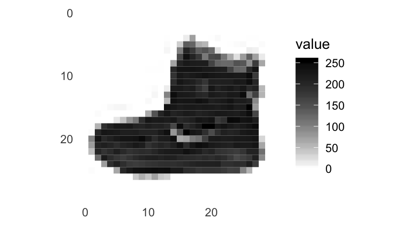
單張圖: 28*28圖點, 256灰階
0 T-shirt/top
1 Trouser
2 Pullover
3 Dress
4 Coat
5 Sandal
6 Shirt
7 Sneaker
8 Bag
9 Ankle boot
10種分類: 標記0~9
Keras R準備資料: Fashion-MNIST資料集
```{r eval=FALSE}
fashion_mnist <- dataset_fashion_mnist()

# 訓練圖片/訓練標籤, 測試圖片/測試標籤
c(train_images, train_labels) %<-% fashion_mnist$train
c(test_images, test_labels) %<-% fashion_mnist$test

class_names = c('T-shirt/top',
                'Trouser',
                'Pullover',
                'Dress',
                'Coat',
                'Sandal',
                'Shirt',
                'Sneaker',
                'Bag',
                'Ankle boot')
```
2. 準備資料:載入
Keras R準備資料: Fashion-MNIST資料集
```{r eval=FALSE}
dim(train_images)
dim(train_labels)
train_labels[1:20]
dim(test_images)
dim(test_labels)

train_images <- train_images / 255
test_images <- test_images / 255
```
2. 準備資料:檢視資料/資料前處理
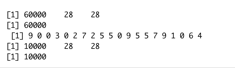
訓練集: 60000萬筆,測試集: 10000筆
Keras R建立模型: Fashion-MNIST資料集
```{r eval=FALSE}
# 建立模型
model <- keras_model_sequential()
model %>%
  layer_flatten(input_shape = c(28, 28)) %>%
  layer_dense(units = 128, activation = 'relu') %>%
  layer_dense(units = 10, activation = 'softmax')

# 編譯模型
model %>% compile(
  optimizer = 'adam',
  loss = 'sparse_categorical_crossentropy',
  metrics = c('accuracy')
)
```
3. 建立深度學習模型: 建立/編譯
隱藏層: 1層
Keras R訓練模型: Fashion-MNIST資料集
```{r eval=FALSE}
# 訓練模型
model %>% fit(train_images, train_labels, epochs = 5)
```
4. 訓練模型
Epoch 1/5
60000/60000 [==============================] - 5s 79us/step - loss: 0.4923 - acc: 0.8273
Epoch 2/5
60000/60000 [==============================] - 4s 70us/step - loss: 0.3740 - acc: 0.8641
Epoch 3/5
60000/60000 [==============================] - 4s 70us/step - loss: 0.3346 - acc: 0.8775
Epoch 4/5
60000/60000 [==============================] - 4s 71us/step - loss: 0.3117 - acc: 0.8861
Epoch 5/5
60000/60000 [==============================] - 4s 75us/step - loss: 0.2931 - acc: 0.8916
Keras R訓練模型: Fashion-MNIST資料集
4. 訓練模型
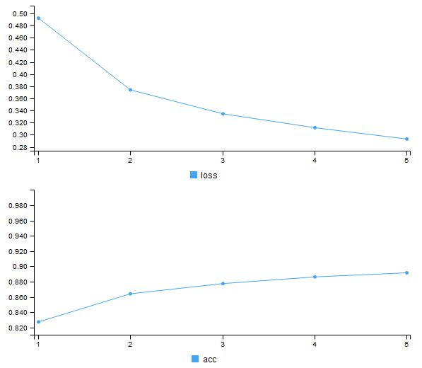
0.8916
0.2931
Keras R評估模型: Fashion-MNIST資料集
```{r eval=FALSE}
# 評估正確性
score <- model %>% evaluate(test_images, test_labels)

cat('Test loss:', score$loss, "\n")
cat('Test accuracy:', score$acc, "\n")
```
5. 評估模型(測試集)
Test loss: 0.3526644
Test accuracy: 0.8737
Keras R運用: Fashion-MNIST資料集
```{r eval=FALSE}
# 檢視一筆預測結果
predictions <- model %>% predict(test_images)  # 10000筆測試集套用模型預測
predictions[1, ]                               # 印出第一筆
answer <- which.max(predictions[1, ]) - 1      # 預測機率最高者 - 1
test_labels[1]                                 # 陣列index:1-10,對應test_labels: 0-9

# 印出25筆預測結果
par(mfcol=c(5,5))
par(mar=c(0, 0, 1.5, 0), xaxs='i', yaxs='i')
for (i in 1:25) {
  img <- test_images[i, , ]
  img <- t(apply(img, 2, rev))
  # subtract 1 as labels go from 0 to 9
  predicted_label <- which.max(predictions[i, ]) - 1
  true_label <- test_labels[i]
  if (predicted_label == true_label) {
    color <- '#008800'
  } else {
    color <- '#bb0000'
  }
  image(1:28, 1:28, img, col = gray((0:255)/255), xaxt = 'n', yaxt = 'n',
        main = paste0(class_names[predicted_label + 1], " (",
                      class_names[true_label + 1], ")"),
        col.main = color)
}
```
Keras R運用: Fashion-MNIST資料集
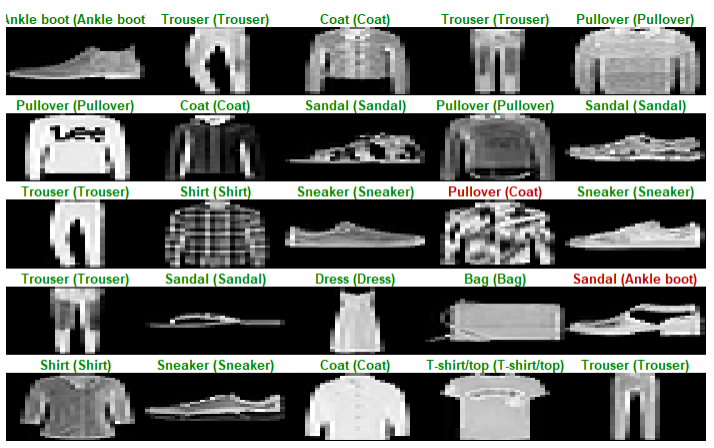
紅色為預測錯誤
Keras R應用: Fashion-MNIST資料集
```{r eval=FALSE}
# 預測新影像
img <- test_images[1, , , drop = FALSE]  # 此處以測試集第一張替代
dim(img)                                 # 28*28矩陣  0~1數值:灰階
predictions <- model %>% predict(img)    # 以模型進行預測
predictions                              # 分類機率串列(1~10)
# 減1 因為標籤為0~9
which.max(predictions)-1                 # 預測答案
class_pred <- model %>% predict_classes(img)
class_pred                               # 標準答案
```
---
title: "Fashion MINST"
output: html_document
---
## 安裝 Keras R (rstudio/keras)
```{r eval=FALSE}
if(!"devtools" %in% installed.packages())
install.packages("devtools");
if(!"keras" %in% installed.packages()) {
require(devtools);
install_github("rstudio/keras");
}
if(!"ggplot2" %in% installed.packages()) {
install.packages("ggplot2");
}
```
```{r eval=FALSE}
## 1.載入Keras
library(keras)
# install_keras()
```
```{r eval=FALSE}
## 2.準備資料:載入fashion mnist資料庫: 含訓練集/測試
fashion_mnist <- dataset_fashion_mnist()
# 訓練圖片/訓練標籤, 測試圖片/測試標籤
c(train_images, train_labels) %<-% fashion_mnist$train
c(test_images, test_labels) %<-% fashion_mnist$test
class_names = c('T-shirt/top',
'Trouser',
'Pullover',
'Dress',
'Coat',
'Sandal',
'Shirt',
'Sneaker',
'Bag',
'Ankle boot')
```
```{r eval=FALSE}
## 3.準備資料:檢視資料/資料前處理
dim(train_images)
dim(train_labels)
train_labels[1:20]
dim(test_images)
dim(test_labels)
train_images <- train_images / 255
test_images <- test_images / 255
```
```{r eval=FALSE}
# 建立模型
model <- keras_model_sequential()
model %>%
layer_flatten(input_shape = c(28, 28)) %>%
layer_dense(units = 128, activation = 'relu') %>%
layer_dense(units = 10, activation = 'softmax')
# 編譯模型
model %>% compile(
optimizer = 'adam',
loss = 'sparse_categorical_crossentropy',
metrics = c('accuracy')
)
```
```{r eval=FALSE}
# 訓練模型
model %>% fit(train_images, train_labels, epochs = 5)
# 評估正確性
score <- model %>% evaluate(test_images, test_labels)
cat('Test loss:', score$loss, "\n")
cat('Test accuracy:', score$acc, "\n")
```
```{r eval=FALSE}
# 檢視一筆預測結果
predictions <- model %>% predict(test_images) # 10000筆測試集套用模型預測
predictions[1, ] # 印出第一筆
answer <- which.max(predictions[1, ]) - 1 # 預測機率最高者 - 1
test_labels[1] # 陣列index:1-10,對應test_labels: 0-9
# 印出25筆預測結果
par(mfcol=c(5,5))
par(mar=c(0, 0, 1.5, 0), xaxs='i', yaxs='i')
for (i in 1:25) {
img <- test_images[i, , ]
img <- t(apply(img, 2, rev))
# subtract 1 as labels go from 0 to 9
predicted_label <- which.max(predictions[i, ]) - 1
true_label <- test_labels[i]
if (predicted_label == true_label) {
color <- '#008800'
} else {
color <- '#bb0000'
}
image(1:28, 1:28, img, col = gray((0:255)/255), xaxt = 'n', yaxt = 'n',
main = paste0(class_names[predicted_label + 1], " (",
class_names[true_label + 1], ")"),
col.main = color)
}
```
```{r eval=FALSE}
# 預測新影像
img <- test_images[1, , , drop = FALSE] # 此處以測試集第一張替代
dim(img) # 28*28矩陣 0~1數值:灰階
predictions <- model %>% predict(img) # 以模型進行預測
predictions # 分類機率串列(1~10)
# 減1 因為標籤為0~9
which.max(predictions)-1 # 預測答案
class_pred <- model %>% predict_classes(img)
class_pred # 標準答案
```完整範例
Keras R修改(1/2)
```{r eval=FALSE}
# 建立模型
model <- keras_model_sequential()
model %>%
  layer_flatten(input_shape = c(28, 28)) %>%
  layer_dense(units = 128, activation = 'relu') %>%
  layer_dense(units = 10, activation = 'softmax')
```
隱藏層: 1層
增加 layer_dense() 全連接層, layer_dropout() 降低模型複雜度
```{r eval=FALSE}
# 訓練模型
model %>% fit(train_images, train_labels, epochs = 5)
```
❶修改模型
❷調整訓練參數
調整fit()參數:epochs(回合數), batch_size預設值32
Keras R修改(2/2)
```{r eval=FALSE}
# 編譯模型
model %>% compile(
  optimizer = 'adam',
  loss = 'sparse_categorical_crossentropy',
  metrics = c('accuracy')
)
```
❸修改優化參數
optimizer: 優化器(優化演算法)
loss: 損失函數
Keras R 優化函式(optimization)
優化過程: 迭代進行
- Epochs參數
- 優化演算法
梯度搜尋
找出最適函數
優化目的: 找出最適函數
- 誤差最小
- 函數: 直線/曲線
誤差? 損失函數
Keras R 損失函數(loss function)
損失函數:
- 計算目前的「最適函數」與資料點的誤差
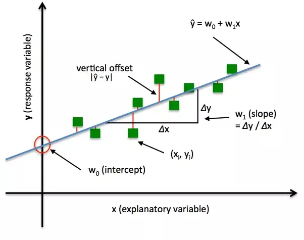

均方根誤差

絕對誤差

平方和誤差
Keras R 優化函式(optimization)
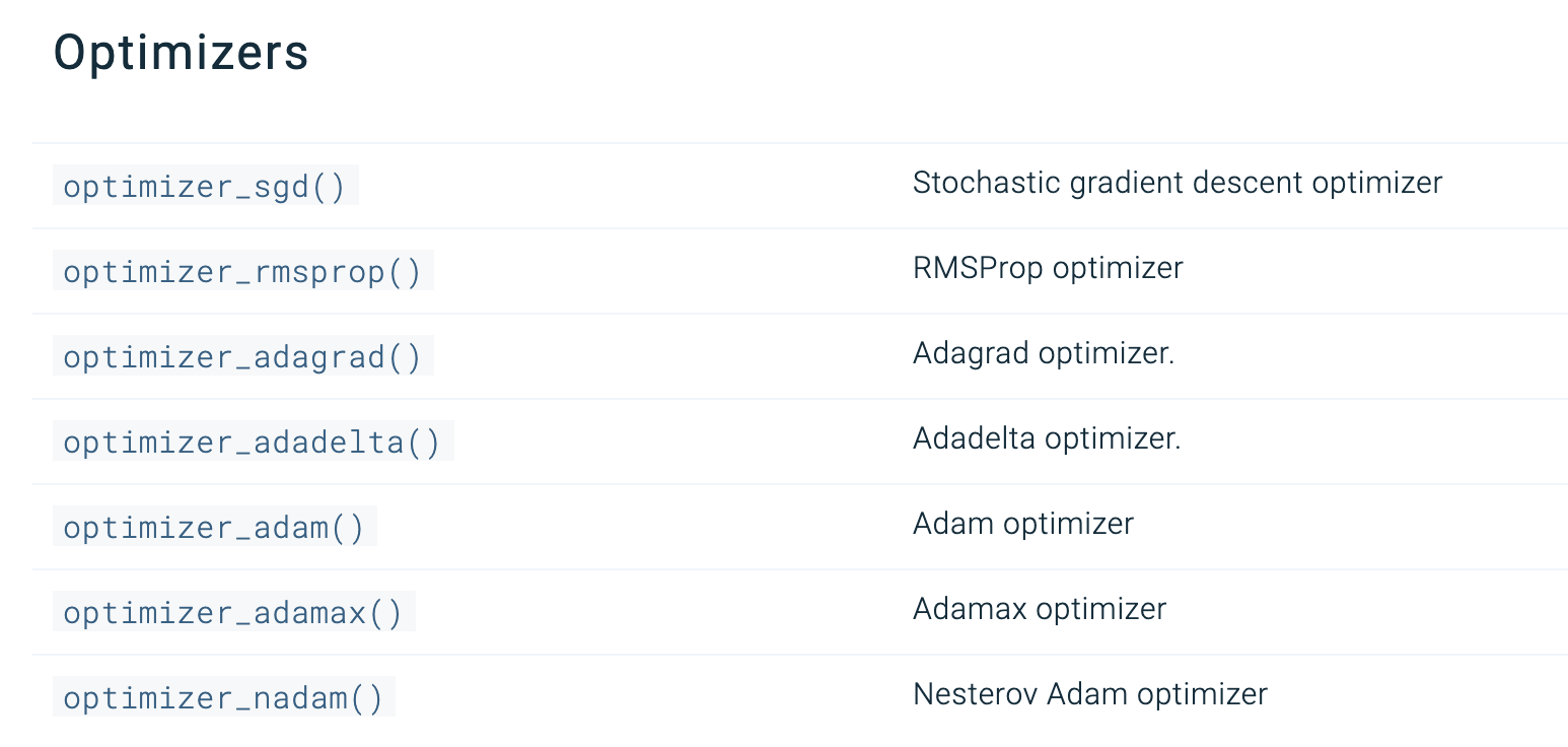
Keras R 優化器
model %>% compile(
  optimizer = 'adam',
  loss = 'sparse_categorical_crossentropy',
  metrics = c('accuracy')
)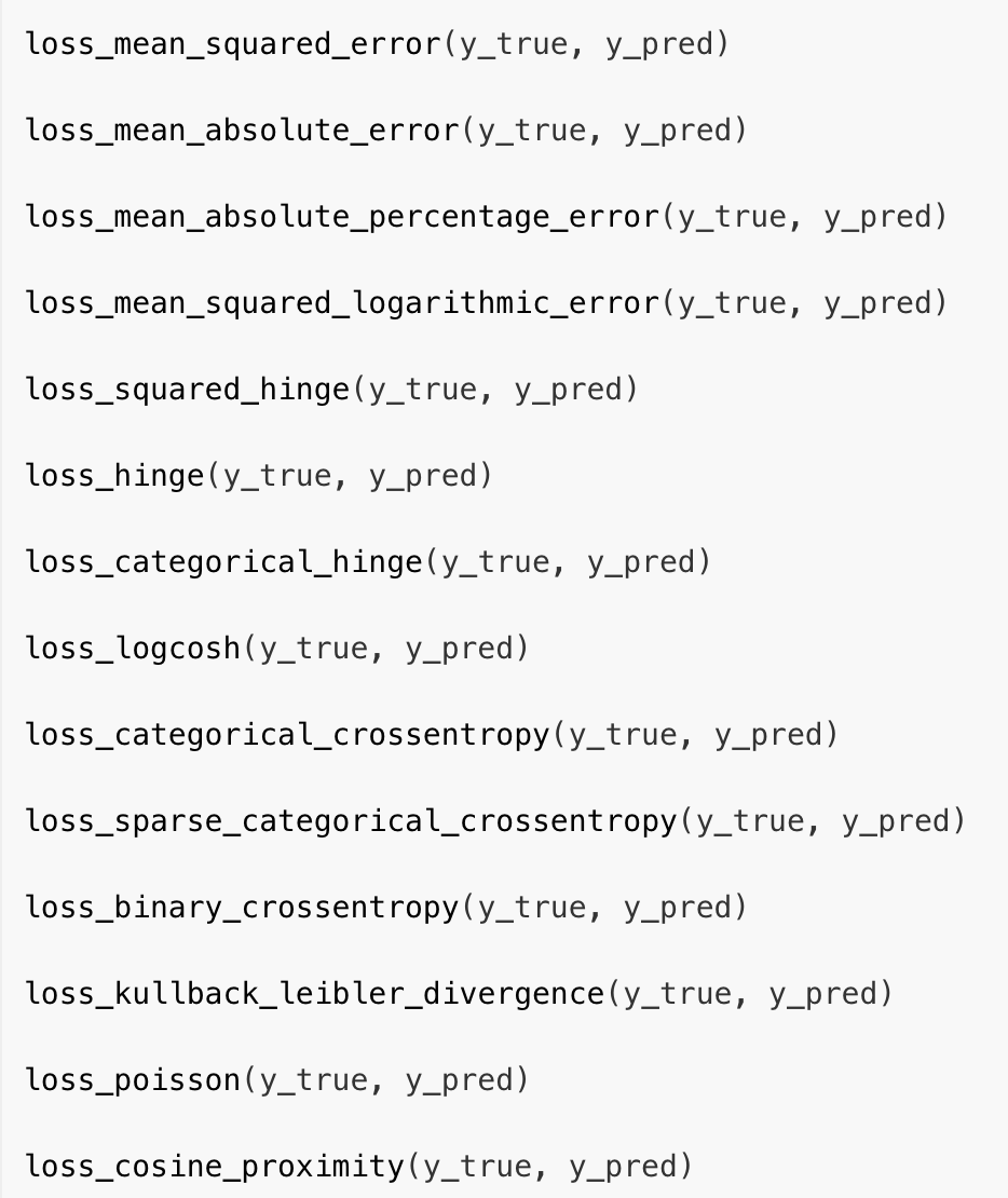
Keras R 損失函數(loss function)
只能用於分類問題
卷積神經網路CNN理論
Convolutional Neural Network (CNN)
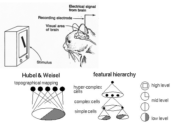
模仿人腦視覺神經運作
1962, Hubel & Weisel的實驗
神經元可辨識不同形狀(低階特徵)
低階組合辨識高階特徵(例:人臉)
組合
特徵階層
卷積神經網路CNN理論
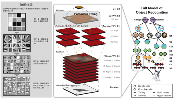
Convolutional Neural Network (CNN)
(1) 底層逐層學習低階特徵 (2)由低階特徵組合出高階特徵
像素明暗
形狀邊緣
更多形狀物體
哪些形狀物件可辨識人臉
低階
高階
低階
高階
卷積神經網路CNN適用範圍

Convolutional Neural Network (CNN)
(1) 適用於classification tasks
(2) 輸入為: images, video, text, or sound
特徵學習
卷積神經網路CNN架構
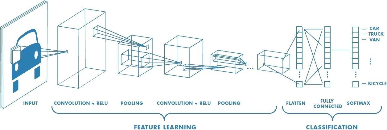
Convolutional Neural Network (CNN)
(1) 卷積層 (convolution layer): 學習特徵
(2) 池化層 (pooling Layer): 取樣 subsampling
(3) 全連接層: 原multi-layer perceptron
卷積層
池化層
特徵學習
分類模型
全連接層
卷積層
池化層
原來之multilayer perceptron網路
卷積神經網路CNN架構-卷積層
Convolutional Neural Network (CNN)
(1) 卷積層 (convolution layer): 學習特徵
2.決定使用3*3矩陣(濾鏡)
1. 輸入圖片5*5
3.產生3*3 特徵圖
(5-3+1)
Kernel 或稱 Filter: 就是濾鏡的功能
濾鏡的效果: 用於邊緣偵測的情形
卷積神經網路CNN架構-池化層
Convolutional Neural Network (CNN)
(2) 池化層 (pooling Layer): 取樣 subsampling
1.N*N特徵圖
3.產生2*2 池化特徵圖
2.使用N/2*N/2取樣
最大池化: 取樣該區最大值➞代表值
卷積神經網路CNN架構
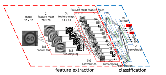
Convolutional Neural Network (CNN)
特徵擷取: 兩層卷積層+兩層池化層 (c1)
2.決定使用5*5矩陣
1. 輸入圖片32*32
3. C1產生28*28 特徵圖
(32-5+1)
4. 2*2取樣
5. S1產生14*14特徵圖
6. C2產生10*10特徵圖
(14-5+1)
7. 2*2取樣
8. S1產生5*5特徵圖
(28/2)
(10/2)
9. 輸入層:5*5特徵圖
卷積神經網路CNN: MNIST
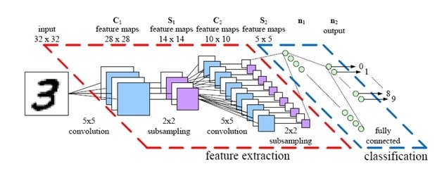
Convolutional Neural Network (CNN)
卷積神經網路CNN: MNIST
Convolutional Neural Network (CNN)
平坦層
隱藏層
輸出層
10個濾鏡
20個濾鏡
MNIST資料集
訓練集:60000筆
測試集:10000筆
3維陣列(images筆數, 圖寬, 圖高)
圖:28*28 共784圖點

60000 rows
28 columns
.
.
.
28 slices
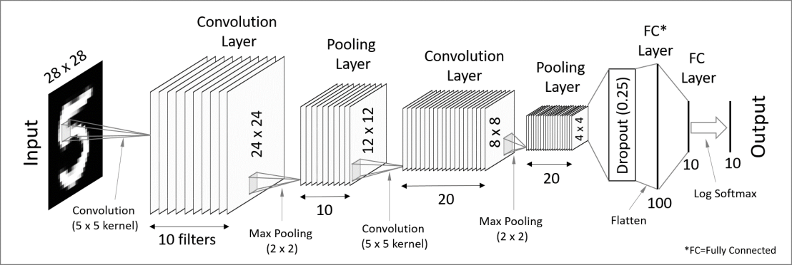
MNIST資料集CNN:模型設定
model <- keras_model_sequential() %>%
  # 卷積層C1
  layer_conv_2d(filters = 32, kernel_size = c(3,3), activation = 'relu',
                input_shape = input_shape) %>%
  # 卷積層C2
  layer_conv_2d(filters = 64, kernel_size = c(3,3), activation = 'relu') %>%
  # 池化層S2
  layer_max_pooling_2d(pool_size = c(2, 2)) %>%
  layer_dropout(rate = 0.25) %>%
  # 平坦層 12*12﹡64 節點
  layer_flatten() %>%
  # 隱藏層
  layer_dense(units = 128, activation = 'relu') %>%
  layer_dropout(rate = 0.5) %>%
  # 輸出層
  layer_dense(units = num_classes, activation = 'softmax')
卷積層C1: 輸出32圖層, 3*3矩陣, 輸入層 (28, 28, 1圖層)
卷積層C2: 輸出64圖層, 3*3矩陣
池化層S2: 縮減圖點成12*12, 仍是64圖層
MNIST資料集CNN:模型設定
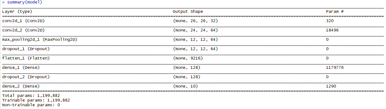
12*12*24個節點
(9216+1) * 128
(128+1) * 10
(3*3+1)*32個
32*(24*24)+64
MNIST資料集CNN:評估設定
# Compile model
model %>% compile(
  loss = loss_categorical_crossentropy,
  optimizer = optimizer_adadelta(),
  metrics = c('accuracy')
)
MNIST資料集CNN:訓練階段
# Train model
model %>% fit(
  x_train, y_train,
  batch_size = batch_size,
  epochs = epochs,
  validation_split = 0.2
)
# Data Preparation ------------------------------------
batch_size <- 128 # 分批大小
num_classes <- 10 # 輸出層節點數0~9機率
epochs <- 12 # 訓練回合數
卷積神經網路CNN:完整範例
```{r eval=FALSE}
library(keras)

# Data Preparation -----------------------------------------------------

batch_size <- 128   # 分批大小
num_classes <- 10   # 輸出層節點數0~9機率
epochs <- 12        # 訓練回合數

# 圖片圖點數 28*28
img_rows <- 28
img_cols <- 28

# 讀取資料集, 分成訓練集,測試集
mnist <- dataset_mnist()
x_train <- mnist$train$x
y_train <- mnist$train$y
x_test <- mnist$test$x
y_test <- mnist$test$y

# 將原本資料集的三維陣列,轉為矩陣
x_train <- array_reshape(x_train, c(nrow(x_train), img_rows, img_cols, 1))
x_test <- array_reshape(x_test, c(nrow(x_test), img_rows, img_cols, 1))
input_shape <- c(img_rows, img_cols, 1)  ## 輸入圖片 28*28* 1圖層

# 將圖點灰階0~255 轉成 [0,1] range
x_train <- x_train / 255
x_test <- x_test / 255

cat('x_train_shape:', dim(x_train), '\n')
cat(nrow(x_train), 'train samples\n')
cat(nrow(x_test), 'test samples\n')

# 將答案轉成矩陣
y_train <- to_categorical(y_train, num_classes)
y_test <- to_categorical(y_test, num_classes)

# Define Model -----------------------------------------------------------

# Define model
model <- keras_model_sequential() %>%
  layer_conv_2d(filters = 32, kernel_size = c(3,3), activation = 'relu',
                input_shape = input_shape) %>%
  layer_conv_2d(filters = 64, kernel_size = c(3,3), activation = 'relu') %>%
  layer_max_pooling_2d(pool_size = c(2, 2)) %>%
  layer_dropout(rate = 0.25) %>%
  layer_flatten() %>%
  layer_dense(units = 128, activation = 'relu') %>%
  layer_dropout(rate = 0.5) %>%
  layer_dense(units = num_classes, activation = 'softmax')

# Compile model
model %>% compile(
  loss = loss_categorical_crossentropy,
  optimizer = optimizer_adadelta(),
  metrics = c('accuracy')
)

# Train model
model %>% fit(
  x_train, y_train,
  batch_size = batch_size,
  epochs = epochs,
  validation_split = 0.2
)

scores <- model %>% evaluate(
  x_test, y_test, verbose = 0
)

# Output metrics
cat('Test loss:', scores[[1]], '\n')
cat('Test accuracy:', scores[[2]], '\n')
```
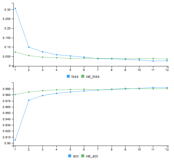
卷積神經網路CNN:訓練結果
Train on 48000 samples, validate on 12000 samples
Epoch 1/12
48000/48000 [==============================] - 141s 3ms/step - loss: 0.3055 - acc: 0.9050 - val_loss: 0.0725 - val_acc: 0.9803
Epoch 2/12
48000/48000 [==============================] - 148s 3ms/step - loss: 0.0989 - acc: 0.9709 - val_loss: 0.0539 - val_acc: 0.9845
Epoch 3/12
48000/48000 [==============================] - 145s 3ms/step - loss: 0.0737 - acc: 0.9787 - val_loss: 0.0455 - val_acc: 0.9868
Epoch 4/12
48000/48000 [==============================] - 146s 3ms/step - loss: 0.0586 - acc: 0.9823 - val_loss: 0.0427 - val_acc: 0.9881
Epoch 5/12
48000/48000 [==============================] - 148s 3ms/step - loss: 0.0519 - acc: 0.9846 - val_loss: 0.0393 - val_acc: 0.9887
Epoch 6/12
48000/48000 [==============================] - 149s 3ms/step - loss: 0.0458 - acc: 0.9863 - val_loss: 0.0398 - val_acc: 0.9891
Epoch 7/12
48000/48000 [==============================] - 114s 2ms/step - loss: 0.0375 - acc: 0.9879 - val_loss: 0.0396 - val_acc: 0.9880
Epoch 8/12
48000/48000 [==============================] - 113s 2ms/step - loss: 0.0363 - acc: 0.9886 - val_loss: 0.0390 - val_acc: 0.9892
Epoch 9/12
48000/48000 [==============================] - 113s 2ms/step - loss: 0.0336 - acc: 0.9895 - val_loss: 0.0372 - val_acc: 0.9905
Epoch 10/12
48000/48000 [==============================] - 122s 3ms/step - loss: 0.0306 - acc: 0.9907 - val_loss: 0.0375 - val_acc: 0.9899
Epoch 11/12
48000/48000 [==============================] - 138s 3ms/step - loss: 0.0255 - acc: 0.9919 - val_loss: 0.0381 - val_acc: 0.9899
Epoch 12/12
48000/48000 [==============================] - 139s 3ms/step - loss: 0.0264 - acc: 0.9917 - val_loss: 0.0350 - val_acc: 0.9903卷積神經網路CNN:訓練結果
卷積神經網路CNN:測試結果
> # Output metrics
> cat('Test loss:', scores[[1]], '\n')
Test loss: 0.02830164
> cat('Test accuracy:', scores[[2]], '\n')
Test accuracy: 0.9909
MLP 測試正確率為 98.18%
CNN為99.09%
行動技術與應用
By Leuo-Hong Wang
行動技術與應用
Lesson 9: Convolutional Neural Network


