行動技術與應用
Lesson 10: More Examples
波士頓房價預測資料敘述
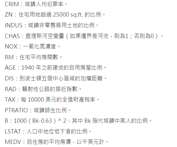

13個輸入變量
1個輸出變量
波士頓房價預測資料敘述
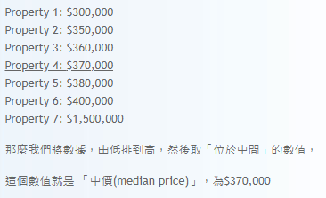
訓練模型:預測房價的「中位數」
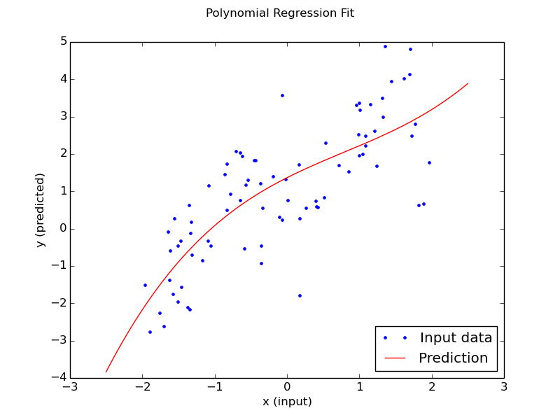
迴歸 (regression)
given: N輸入變數
output: 數值
波士頓房價預測訓練集/測試集
 0.00632  18.00   2.310  0  0.5380  6.5750  65.20  4.0900   1  296.0  15.30 396.90   4.98  24.00
 0.02731   0.00   7.070  0  0.4690  6.4210  78.90  4.9671   2  242.0  17.80 396.90   9.14  21.60
 0.02729   0.00   7.070  0  0.4690  7.1850  61.10  4.9671   2  242.0  17.80 392.83   4.03  34.70
 0.03237   0.00   2.180  0  0.4580  6.9980  45.80  6.0622   3  222.0  18.70 394.63   2.94  33.40
 0.06905   0.00   2.180  0  0.4580  7.1470  54.20  6.0622   3  222.0  18.70 396.90   5.33  36.20
 0.02985   0.00   2.180  0  0.4580  6.4300  58.70  6.0622   3  222.0  18.70 394.12   5.21  28.70
 ...
資料集:共606筆
訓練集:404筆 測試集:102筆
問題:
訓練樣本少!
欄位尺度互不相同,有介於0~1之間的比值,也有其他尺度。
波士頓房價預測資料準備
```{r}
library(keras)

dataset <- dataset_boston_housing()
# multiple assignment from dataset to variables on the left hand side
c(c(train_data, train_targets), c(test_data, test_targets)) %<-% dataset

# Compactly display training data
str(train_data)

str(test_data)
```
資料集:
資料來源 dataset_boston_housing()
dataset$train$x,..., dataset$test$y
# 讀取資料集, 分成訓練集,測試集
mnist <- dataset_mnist()
x_train <- mnist$train$x
y_train <- mnist$train$y
x_test <- mnist$test$x
y_test <- mnist$test$y波士頓房價預測資料準備
```{r}
mean <- apply(train_data, 2, mean) # 計算平均值, 2為按列計算, 套用於每個feature
std <- apply(train_data, 2, sd)    # 計算標準差

train_data <- scale(train_data, center = mean, scale = std) # 正規化
test_data <- scale(test_data, center = mean, scale = std)
```
此處正規化是 (數值-平均值)/標準差。
正規化後數值以0為中心,且大部分數值落在一個標準差內。
R的scale()函式,恰可完成此調整動作。
欄位尺度互不相同:NN學習效能將大打折扣,需正規化處理
波士頓房價預測網路模型建置
```{r}
# build_model function
build_model <- function() {
  model <- keras_model_sequential() %>%
    layer_dense(units = 64, activation = "relu",
                input_shape = dim(train_data)[[2]]) %>%
    layer_dense(units = 64, activation = "relu") %>%
    layer_dense(units = 1)

  model %>% compile(
    optimizer = "rmsprop",
    loss = "mse",
    metrics = c("mae")
  )
}
```
輸入層:dim(train_data)[[2]] 13個輸入值
兩個隱藏層:各64個節點。 此舉是為了避免overfitting
輸出層:單一節點,無設定激勵函式,「線性迴歸」的標準設定方式。
訓練資料極少:網路不宜太大。
-最佳化:rmsprop
套用移動平均數概念
適用於小樣本學習
-損失函數:`mse`
均方誤差
迴歸問題廣泛使用
-指標使用: `mae`
Mean Absolute Error
波士頓房價預測網路模型建置
波士頓房價預測交叉驗證
```{r, echo=TRUE, results='hide'}
k <- 4    # 分成4份
indices <- sample(1:nrow(train_data))  # sample() 隨機產生rows序號
folds <- cut(indices, breaks = k, labels = FALSE)  # 將rows編號對應到1~4區間

num_epochs <- 100
all_scores <- c()
for (i in 1:k) {
  cat("處理fold #", i, "\n")
  # 準備驗證集: 第i份為驗證集
  val_indices <- which(folds == i, arr.ind = TRUE)
  val_data <- train_data[val_indices,]
  val_targets <- train_targets[val_indices]
  # 準備訓練集: 第i份以外全部是訓練集
  partial_train_data <- train_data[-val_indices,]
  partial_train_targets <- train_targets[-val_indices]
  # 呼叫先前所寫的build_model()
  model <- build_model()
  # 訓練網路模型 (in silent mode, verbose=0)
  model %>% fit(partial_train_data, partial_train_targets,
                epochs = num_epochs, batch_size = 1, verbose = 0)
  # 使用驗證集評估訓練好的網路模型
  results <- model %>% evaluate(val_data, val_targets, verbose = 0)
  all_scores <- c(all_scores, results$mean_absolute_error)
}
```
訓練資料極少:可使用交叉驗證,尋求較正確的模型評估方式。
-使用交叉驗證(K-fold cross-validation)
訓練資料分成K份(K通常為4或5)
建立K個相同的網路模型
(K-1)份訓練資料
剩下的那一份則作為驗證資料
驗證分數: K個分數的平均
波士頓房價預測參數調整
```{r}
# Some memory clean-up
K <- backend()
K$clear_session()
```
```{r, echo=TRUE, results='hide'}
num_epochs <- 500
all_mae_histories <- NULL
for (i in 1:k) {
  cat("處理fold #", i, "\n")
  # 準備驗證集: 第i份為驗證集
  val_indices <- which(folds == i, arr.ind = TRUE)
  val_data <- train_data[val_indices,]
  val_targets <- train_targets[val_indices]
  # 準備訓練集: 第i份以外全部是訓練集
  partial_train_data <- train_data[-val_indices,]
  partial_train_targets <- train_targets[-val_indices]
  # 呼叫先前所寫的build_model()
  model <- build_model()
  # 訓練網路模型 (in silent mode, verbose=0)
  history <- model %>% fit(
    partial_train_data, partial_train_targets,
    validation_data = list(val_data, val_targets),
    epochs = num_epochs, batch_size = 1, verbose = 0
  )
  mae_history <- history$metrics$val_mean_absolute_error  #記錄訓練過程
  all_mae_histories <- rbind(all_mae_histories, mae_history)
}
```
驗證結果不理想?調整參數,例如epochs從100上調至500
紀錄訓練資料
波士頓房價預測參數調整
計算每一epoch的MAE scores(4個folds平均值)
```{r}
average_mae_history <- data.frame(
  epoch = seq(1:ncol(all_mae_histories)),
  validation_mae = apply(all_mae_histories, 2, mean)
)
```
圖形繪出如下:
```{r}
library(ggplot2)
ggplot(average_mae_history, aes(x = epoch, y = validation_mae)) + geom_line()
```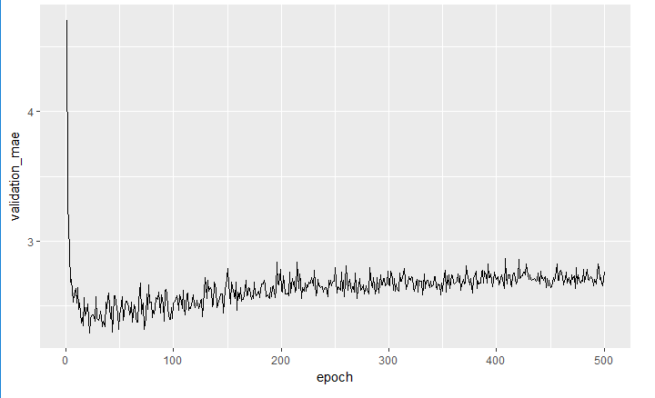
波士頓房價預測參數調整
圖形變化大,改用 `geom_smooth()`,簡化圖形:
```{r}
ggplot(average_mae_history, aes(x = epoch, y = validation_mae)) + geom_smooth()
```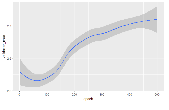
70 epochs以後的驗證值並未持續改善
故epochs改成80
其他參數也需進行調校,最後才能得到最佳模型。
波士頓房價預測參數調整
最後,假設已找到可接受的模型,再進行訓練,並套用測試集:
```{r, echo=FALSE, results='hide'}
# Get a fresh, compiled model.
model <- build_model()

# Train it on the entirety of the data.
model %>% fit(train_data, train_targets,
          epochs = 80, batch_size = 16, verbose = 0)

result <- model %>% evaluate(test_data, test_targets)
```

```{r}
result
```
波士頓房價預測
```{r setup, include=FALSE}
knitr::opts_chunk$set(warning = FALSE, message = FALSE)
if(!"ggplot2" %in% installed.packages())
install.packages('ggplot2')
# 安裝'devtools' package:方便從github安裝套件
if(!"devtools" %in% installed.packages())
install.packages('devtools')
require(devtools)
# install tensorflow(如果你要tensorflow的話)
devtools::install_github("rstudio/tensorflow")
# installing keras(如果你要keras的話)
devtools::install_github("rstudio/keras")
```
## Boston Housing Price資料集
1970年代Boston市郊房價中位數預測
訓練資料集不大,共506筆,分為訓練集404筆,測試集102筆。
此外各特徵欄位的尺度並不相同,有些為介於0~1之間的比值,有些則是1~12或是0~100的尺度。
資料集如下:
```{r}
library(keras)
dataset <- dataset_boston_housing()
# multiple assignment from dataset to variables on the left hand side
c(c(train_data, train_targets), c(test_data, test_targets)) %<-% dataset
```
```{r}
# Compactly display training data
str(train_data)
```
```{r}
str(test_data)
```
前13個數值是輸入變數
第14個數值是房價,單位是千元。
目標是學習房價的「中位數」(the median values)。
```{r}
str(train_targets)
```
房價大多介於 \$10,000 and \$50,000.之間.
## 資料準備
當輸入值為各種不同的數值範圍時,NN學習效能將大打折扣。因此,必須將輸入資料正規化。
此處正規化是 (數值-平均值)/標準差。正規化後數值以0為中心,且大部分數值落在一個標準差內。
R的scale()函式,恰可完成此調整動作。
```{r}
mean <- apply(train_data, 2, mean) # 計算平均值, 2為按列計算, 套用於每個feature
std <- apply(train_data, 2, sd) # 計算標準差
train_data <- scale(train_data, center = mean, scale = std) # 正規化
test_data <- scale(test_data, center = mean, scale = std)
```
## 網路模型建置
由於訓練資料極少,故網路不宜太大。此處使用兩個隱藏層,各64個節點。 此舉是為了避免overfitting。
```{r}
# build_model function
build_model <- function() {
model <- keras_model_sequential() %>%
layer_dense(units = 64, activation = "relu",
input_shape = dim(train_data)[[2]]) %>%
layer_dense(units = 64, activation = "relu") %>%
layer_dense(units = 1)
model %>% compile(
optimizer = "rmsprop",
loss = "mse",
metrics = c("mae")
)
}
```
輸出層為單一節點,且無設定激勵函式,此線性設定方式是解「線性迴歸」預測問題的標準設定方式。
損失函式採用:`mse` loss function --均方誤差( Mean Squared Error)。也是迴歸問題廣泛使用的loss function。
指標使用: `mae`。Mean Absolute Error。
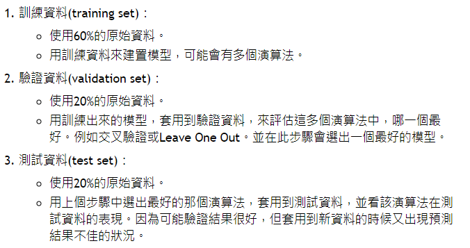
## Validating our approach using K-fold validation
使用交叉驗證方式(K-fold cross-validation). 將訓練資料分成K份(K通常為4或5)。 接著建立K個相同的網路模型,並將(K-1)份訓練資料丟進去訓練,剩下的那一份則作為驗證用途。因此,網路模型的驗證分數就是 K個分數的平均。
K-fold cross-validation 做法如下:
```{r, echo=TRUE, results='hide'}
k <- 4 # 分成4份
indices <- sample(1:nrow(train_data)) # sample() 隨機產生rows序號
folds <- cut(indices, breaks = k, labels = FALSE) # 將rows編號對應到1~4區間
num_epochs <- 100
all_scores <- c()
for (i in 1:k) {
cat("處理fold #", i, "\n")
# 準備驗證集: 第i份為驗證集
val_indices <- which(folds == i, arr.ind = TRUE)
val_data <- train_data[val_indices,]
val_targets <- train_targets[val_indices]
# 準備訓練集: 第i份以外全部是訓練集
partial_train_data <- train_data[-val_indices,]
partial_train_targets <- train_targets[-val_indices]
# 呼叫先前所寫的build_model()
model <- build_model()
# 訓練網路模型 (in silent mode, verbose=0)
model %>% fit(partial_train_data, partial_train_targets,
epochs = num_epochs, batch_size = 1, verbose = 0)
# 使用驗證集評估訓練好的網路模型
results <- model %>% evaluate(val_data, val_targets, verbose = 0)
all_scores <- c(all_scores, results$mean_absolute_error)
}
```
```{r}
all_scores
```
```{r}
#k-fold validation取平均值做為評估分數
mean(all_scores)
```
每輪的評估分數差異頗大,故平均值應是較為合理的評估指標。
不過,以平均值評估,訓練出來的模型,其平均誤差大約是$2500,似乎仍偏高(房價介於 \$10,000 to \$50,000. )
Epochs重新調整,由100改為 500 epochs.
```{r}
# 記憶體清除,準備重新訓練
K <- backend()
K$clear_session()
```
```{r, echo=TRUE, results='hide'}
num_epochs <- 500
all_mae_histories <- NULL
for (i in 1:k) {
cat("處理fold #", i, "\n")
# 準備驗證集: 第i份為驗證集
val_indices <- which(folds == i, arr.ind = TRUE)
val_data <- train_data[val_indices,]
val_targets <- train_targets[val_indices]
# 準備訓練集: 第i份以外全部是訓練集
partial_train_data <- train_data[-val_indices,]
partial_train_targets <- train_targets[-val_indices]
# 呼叫先前所寫的build_model()
model <- build_model()
# 訓練網路模型 (in silent mode, verbose=0)
history <- model %>% fit(
partial_train_data, partial_train_targets,
validation_data = list(val_data, val_targets),
epochs = num_epochs, batch_size = 1, verbose = 0
)
mae_history <- history$metrics$val_mean_absolute_error #記錄訓練過程
all_mae_histories <- rbind(all_mae_histories, mae_history)
}
```
計算每一epoch的MAE scores(4個folds平均值)
```{r}
average_mae_history <- data.frame(
epoch = seq(1:ncol(all_mae_histories)),
validation_mae = apply(all_mae_histories, 2, mean)
)
```
圖形繪出如下:
```{r}
library(ggplot2)
ggplot(average_mae_history, aes(x = epoch, y = validation_mae)) + geom_line()
```
圖形變化大,改用 `geom_smooth()`,簡化圖形:
```{r}
ggplot(average_mae_history, aes(x = epoch, y = validation_mae)) + geom_smooth()
```
據此圖形,70 epochs以後的驗證值並未持續改善。
故epochs改成80,其他參數也需進行調校,最後才能得到最佳模型。
最後,假設已找到可接受的模型,再進行訓練,並套用測試集:
```{r, echo=FALSE, results='hide'}
# Get a fresh, compiled model.
model <- build_model()
# Train it on the entirety of the data.
model %>% fit(train_data, train_targets,
epochs = 80, batch_size = 16, verbose = 0)
result <- model %>% evaluate(test_data, test_targets)
```
```{r}
result
```完整範例
波士頓房價預測What we learned
-
迴歸問題:MSE loss function, 與分類問題不同
-
評估指標:'acc'不適用於迴歸問題(改使用'mae')
-
輸出資料尺度不同:需做正規化前處理
-
訓練資料量少:交叉驗證(如K-Fold validation)
-
訓練資料量少:小型網路,較少的隱藏層(1或2層)
遞歸類神經網路
Recurrent Neural Network, RNN
長短期記憶模型(long short-term memory, LSTM)
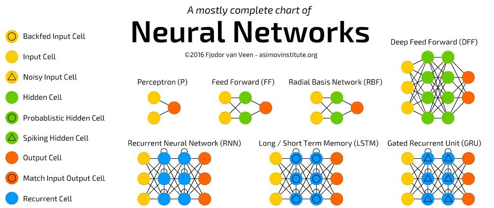
RNN
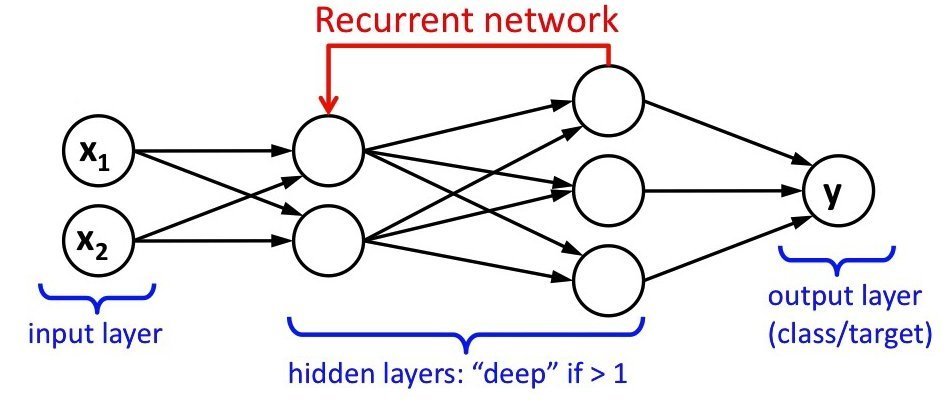
回收循環
今天的預測結果:明天被重新利用,成為明天的「昨日預測」
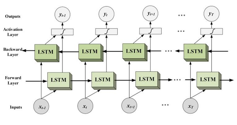
Bidirectional LSTM
IMDb資料集
IMDb: 網路電影資料庫
內容為影評文字
應用:情緒分析(sentiment analysis)/ 意見探勘
50000筆影評,已經詞頻統計、依序編號
訓練集:25000筆
測試集:25000筆
標記:正面 or 負面 評價
模型: RNN-長短期記憶模型
考慮前言後語(同一層的其他神經元),以免斷章取義
長短期記憶: 記憶功能(改善RNN的缺點)
IMDb資料集Keras官網說明
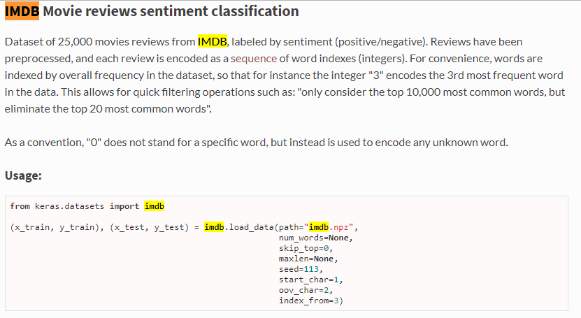
num_words參數
只取最常見的字
IMDb資料集資料前處理參數設定
```{r}
library(keras)

# 只取詞頻排名前20000的字
max_features <- 20000

# 每一篇評論只取100字
# (among top max_features most common words)
maxlen <- 100

batch_size <- 32
```
每篇評論長度需相同,才能餵入NN訓練
資料庫內的字太多,過濾掉不常見的字
NN訓練參數
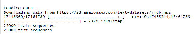
IMDb資料集資料前處理
```{r}
# Load imdb dataset
cat('Loading data...\n')
imdb <- dataset_imdb(num_words = max_features)

# Define training and test sets
x_train <- imdb$train$x
y_train <- imdb$train$y
x_test <- imdb$test$x
y_test <- imdb$test$y

# Output lengths of testing and training sets
cat(length(x_train), 'train sequences\n')
cat(length(x_test), 'test sequences\n')
```
max_features=20000 #取最常出現之前兩萬字
IMDb資料集資料前處理
```{r}
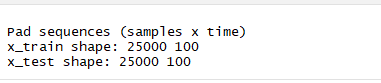
cat('Pad sequences (samples x time)\n')
# Pad training and test inputs
x_train <- pad_sequences(x_train, maxlen = maxlen)
x_test <- pad_sequences(x_test, maxlen = maxlen)
# Output dimensions of training and test inputs
cat('x_train shape:', dim(x_train), '\n')
cat('x_test shape:', dim(x_test), '\n')
```pad_sequences(): 截去多於100以上的字,不足100補0
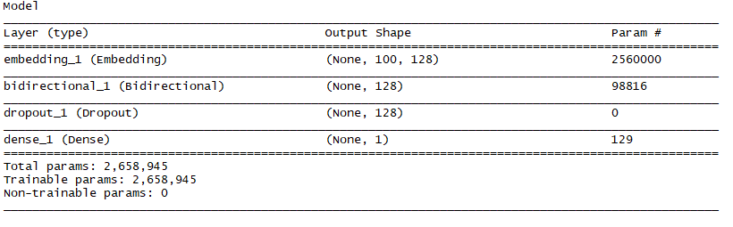
IMDb資料集模型
```{r}
model <- keras_model_sequential()
model %>%
  # Creates dense embedding layer; outputs 3D tensor
  # with shape (batch_size, sequence_length, output_dim)
  layer_embedding(input_dim = max_features,
                  output_dim = 128,
                  input_length = maxlen) %>%
  bidirectional(layer_lstm(units = 64)) %>%
  layer_dropout(rate = 0.5) %>%
  layer_dense(units = 1, activation = 'sigmoid')
```
layer_embedding(): 將文字序號轉成固定長度(output_dim)的向量
layer_lstm(): 長短期記憶模型
bidirectional(): 雙向
IMDb資料集why layer embedding
one hot編碼:非常稀疏
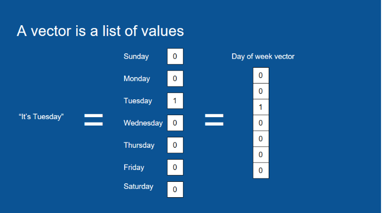
試想:輸入層是20000個詞頻最高的文字,每篇輸入文章最多只取100字,超過19900個輸入是0
以固定長度,如長度5的vector取代
長度:20000 -> 128
IMDb資料集model
```{r}
model <- keras_model_sequential()
model %>%
  # Creates dense embedding layer; outputs 3D tensor
  # with shape (batch_size, sequence_length, output_dim)
  layer_embedding(input_dim = max_features,
                  output_dim = 128,
                  input_length = maxlen) %>%
  bidirectional(layer_lstm(units = 64)) %>%
  layer_dropout(rate = 0.5) %>%
  layer_dense(units = 1, activation = 'sigmoid')
```
IMDb資料集model compile
# Try using different optimizers and different optimizer configs
model %>% compile(
  loss = 'binary_crossentropy',
  optimizer = 'adam',
  metrics = c('accuracy')
)
IMDb資料集訓練
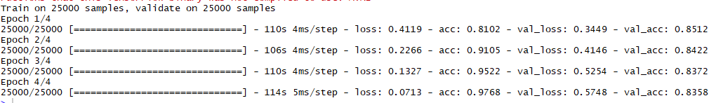
# Train model over four epochs
cat('Train...\n')
model %>% fit(
  x_train, y_train,
  batch_size = batch_size,
  epochs = 4,
  validation_data = list(x_test, y_test)
)IMDb資料集訓練
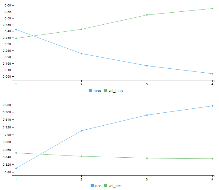
驗證結果不高 約84%
IMDb資料集完整範例
```{r}
#' Train a Bidirectional LSTM on the IMDB sentiment classification task.
#'
#' Output after 4 epochs on CPU: ~0.8146
#' Time per epoch on CPU (Core i7): ~150s.

library(keras)

# Define maximum number of input features
max_features <- 20000

# Cut texts after this number of words
# (among top max_features most common words)
maxlen <- 100

batch_size <- 32
```

```{r}
# Load imdb dataset
cat('Loading data...\n')
imdb <- dataset_imdb(num_words = max_features)

# Define training and test sets
x_train <- imdb$train$x
y_train <- imdb$train$y
x_test <- imdb$test$x
y_test <- imdb$test$y

# Output lengths of testing and training sets
cat(length(x_train), 'train sequences\n')
cat(length(x_test), 'test sequences\n')
```
```{r}
cat('Pad sequences (samples x time)\n')

# Pad training and test inputs
x_train <- pad_sequences(x_train, maxlen = maxlen)
x_test <- pad_sequences(x_test, maxlen = maxlen)

# Output dimensions of training and test inputs
cat('x_train shape:', dim(x_train), '\n')
cat('x_test shape:', dim(x_test), '\n')
```

```{r}
# Initialize model
model <- keras_model_sequential()
model %>%
  # Creates dense embedding layer; outputs 3D tensor
  # with shape (batch_size, sequence_length, output_dim)
  layer_embedding(input_dim = max_features,
                  output_dim = 128,
                  input_length = maxlen) %>%
  bidirectional(layer_lstm(units = 64)) %>%
  layer_dropout(rate = 0.5) %>%
  layer_dense(units = 1, activation = 'sigmoid')

# Try using different optimizers and different optimizer configs
model %>% compile(
  loss = 'binary_crossentropy',
  optimizer = 'adam',
  metrics = c('accuracy')
)

# Train model over four epochs
cat('Train...\n')
model %>% fit(
  x_train, y_train,
  batch_size = batch_size,
  epochs = 4,
  validation_data = list(x_test, y_test)
)
```
更多範例
行動技術與應用
By Leuo-Hong Wang
行動技術與應用
Lesson 10: More Examples


