Book 2. Credit Risk

FRM Part 2

CR 10. Credit Value at Risk

Presented by: Sudhanshu

Module 1. Defining Credit VaR

Module 2. Credit VaR Models

Module 1. Defining Credit VaR

Topic 1. Market VaR vs. Credit VaR

Topic 2. Factors for Calculating Credit VaR

Topic 3. Credit Transition Matrices​

Topic 1. Market VaR vs. Credit VaR

• Definition of Credit VaR: Credit VaR represents the credit loss over a certain time horizon that will not be exceeded given a specific level of confidence
  • Models can consider losses due to defaults, downgrades, and/or credit spread changes.
  • Credit VaR is often used by banks to determine the amount of economic and regulatory capital.
• Market VaR vs. Credit VaR:

  • Time Horizon: Market VaR is typically calculated with a one-day time horizon, whereas credit VaR often uses a one-year time horizon.

  • Calculation Tools: Market VaR primarily uses historical simulation but credit VaR calculations often require more complex modeling tools.

Practice Questions: Q1

Q1. Which of the following statements most accurately reflects the time horizons typically used for market VaR and credit VaR calculations?

A. Both are calculated for one day.

B. Both are calculated for one year.

C. Market risk VaR is calculated over a longer time period than credit risk VaR.

D. Credit risk VaR is calculated over a longer time period than market risk VaR.

Practice Questions: Q1 Answer

Explanation: D is correct.

Market risk VaR is usually calculated over a one-day time horizon, while credit
risk VaR will often use a one-year time horizon.

Topic 2. Factors for Calculating Credit VaR 

• Role of credit correlation: Credit VaR models must incorporate credit correlation, recognizing that defaults across firms are interdependent rather than independent events.

• Economic cycle impact: Strong economic conditions reduce default risk across companies, while downturns increase default risk and correlation.

• Risk amplification: Higher credit correlation during economic stress amplifies portfolio risk for financial institutions.

Practice Questions: Q2

Q2. During a period of slowing economic growth, an analyst will likely identify which of the following trends regarding credit correlation and financial institution risks?

A. A decrease in credit correlation and defaults.

B. An increase in credit correlation and defaults.

C. An increase in credit correlation and a decrease in defaults.

D. A decrease in credit correlation and an increase in defaults.

Practice Questions: Q2 Answer

Explanation: B is correct.

When the economy is slowing, companies are negatively impacted, and defaults will become more prominent. At the same time, credit correlation (which captures the lack of independence between defaults for different companies) increases as well.

Topic 3. Credit Transition Matrices 

• Use in credit VaR: Rating transition matrices are commonly used by financial institutions to model credit VaR by capturing the probability of rating migrations over a given horizon.

• Historical basis: These matrices are derived from historical data and reflect how firms transition between credit rating categories.

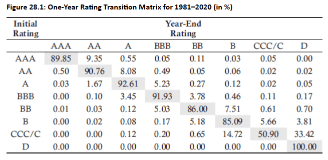
• Market example: A typical example is the one-year rating transition matrix published by S&P, based on issuer ratings observed from 1981 to 2020.

Topic 3. Credit Transition Matrices 

• One-year transition interpretation: Credit rating transition matrices show the highest probabilities along the diagonal, indicating that firms are most likely to retain their current rating over a one-year horizon (e.g., an AA-rated firm has a 90.76% probability of remaining AA).

• Upgrades and downgrades: Off-diagonal entries capture rating migrations, such as upgrades (AA → AAA) and downgrades (AA → A), with probabilities read across the initial rating row.

• Extending the horizon: Multi-year transition matrices are obtained by raising the one-year matrix to the appropriate power (e.g., a three-year matrix is the cube of the one-year matrix), which increases default probabilities and lowers rating-stability probabilities over longer horizons.

• Shortening the horizon: Sub-year transitions are derived by taking roots of the one-year matrix (e.g., fourth root for a three-month horizon), leading to higher probabilities of rating stability and lower default risk.

• Time-horizon effect: Longer horizons imply higher default risk and lower chances of maintaining the same rating, while shorter horizons imply the opposite.

• Independence caveat: The assumption of independence across periods may be violated in practice due to ratings momentum, where recent downgrades increase the likelihood of further downgrades.

Practice Questions: Q3

Q3. Historical data shows that over a one-year period, there is a 91.93% chance that a company rated BBB will keep its rating. What is the percentage chance this rating will remain unchanged over a four-year period?

A. 36.77%.

B. 67.72%.

C. 71.42%.

D. 95.97%.

Practice Questions: Q3 Answer

Explanation: C is correct.

If 91.93% is the likelihood that the company keeps its rating over a one-year period, then there is a 71.42% chance it keeps that rating over a four-year period.
 

Module 2. Credit VaR Models

Topic 1. Vasicek’s Model

Topic 2. Credit Risk Plus Model

Topic 3. CreditMetrics Model

Topic 4. Correlation Model

Topic 5. Credit Spread Risk

Topic 1. Vasicek’s Model

• Purpose of the model: Vasicek’s Gaussian copula is used for loan portfolios to estimate high-percentile outcomes of the default rate distribution.

• Key output: The model produces $\text{WCDR}(T,X)$, the worst-case default rate over horizon $T$ at the $X$th percentile, using PD, credit correlation (ρ) and time horizon T.

ρ\rh

• Formula:​

• Individual loan loss percentile: The Xth percentile loss for a single loan is computed as the product of the worst-case default rate (WCDR), exposure at default (EAD), and loss given default (LGD).

• Large portfolio approximation: For a portfolio with a large number of small loans, the Xth percentile of the loss distribution can be approximated using an aggregate portfolio-level formula.

  •  
  •  
•  

Topic 1. Vasicek Model

• Purpose of the model: Vasicek’s Gaussian copula is used for loan portfolios to estimate high-percentile outcomes of the default rate distribution.

• Key output: The model produces $\text{WCDR}(T,X)$, the worst-case default rate over horizon $T$ at the $X$th percentile, using PD, credit correlation (ρ) and time horizon T.

  •  

  •   

• Individual loan loss percentile: The Xth percentile loss for a single loan is computed as the product of the worst-case default rate (WCDR), exposure at default (EAD), and loss given default (LGD).

• Large portfolio approximation: For a portfolio with a large number of small loans, the Xth percentile of the loss distribution can be approximated using an aggregate portfolio-level formula.

  •  

  •  

Topic 1. Vasicek Model

• Credit Correlation (ρ)

  • Estimation of credit correlation (ρ): In Vasicek’s model, ρ should approximate the correlation between firms’ returns, such as ROA or ROE, and portfolio-level ρ can be estimated using the average correlation of company ROEs.

  • Use of proxies: When firms are not publicly traded, average correlations of similar publicly traded companies can be used as a proxy for estimating ρ.

  • Model limitation: A key limitation of Vasicek’s model is that it does not capture tail correlation, a weakness that can be addressed using alternative modeling approaches.

Practice Questions: Q1

Q1. Company A has an ROE of 8%, while Company B has an ROE of 6%. The average correlation between the two is 0.24, and both companies are publicly traded. The credit correlation      most likely used in Vasicek’s Gaussian copula model will be closest to:

A. 0.12.

B. 0.24.

C. 0.48.

D. 0.76.

Practice Questions: Q1 Answer

Explanation: B is correct.

The average correlation between company ROEs can be used to determine   . Because the average correlation is given as 0.24, that is the most likely correlation used in Vasicek’s model.

Topic 2. Credit Risk Plus Model

• Overview: Developed by Credit Suisse Financial Products, the Credit Risk Plus (also known as CreditRisk+) model is a credit VaR calculation methodology.
• Default Probability: Assuming independent defaults, a binomial distribution can be used to estimate the number of defaults.
• The probability of m defaults with n loans and a PD of q for each loan is:

  • ​

  •  

• For a small probability of default and a large number of loans, a Poisson distribution can be used:

  • ​

  •  

• Assumption on defaults: When $q$ is unknown, the expected number of defaults $qn$ is assumed to follow a gamma distribution with mean $\mu$ and standard deviation $\rho$.

  • Under this assumption, the Poisson distribution for defaults transforms into a negative binomial distribution, as follows

  • ​​
  •  
    •  
    •  

Topic 2. Credit Risk Plus Model

• Effect of ρ on default distribution: As ρ decreases, the negative binomial distribution converges toward the Poisson distribution, while higher values of ρ increase the probability of observing a large number of defaults.

• Role of Monte Carlo simulation: Monte Carlo methods incorporate default rate uncertainty by allowing default rates to depend on prior-year defaults or economic conditions, rather than assuming independence across years.

• Implications for loss distribution: Rising default rate uncertainty increases default correlation, raising the likelihood of extreme default outcomes and producing a positively skewed loss distribution.

• Limitations of Vasicek and Credit Risk Plus Models: Both Vasicek’s and Credit Risk Plus models account for only defaults and not downgrades.

Topic 3. CreditMetrics Model

• Overview: The CreditMetrics model, from JPMorgan, was designed to account for both  defaults and downgrades.
  • It uses a rating transition matrix, with ratings from internal bank data or external credit rating agencies.
• Monte Carlo Simulation: Monte Carlo simulation is used for one-year credit VaR calculations for portfolios with multiple counterparties.

  • Each simulation trial determines the counterparty credit ratings at the end of one year and calculates the credit loss for each counterparty.

  • If a default occurs, the loss equals the EAD multiplied by the LGD.

  • If there is no default, the credit loss is the value of all transactions with that counterparty at year-end.

  • The term structure of credit spreads for each rating category is needed for these calculations. This term structure is assumed to be either the same as what is observable in the market or based on a credit spread index.​

• ​Simulation assumption: In a CreditMetrics simulation trial, assume no default occurs during the first year.

• Default probabilities: The one-year credit spread term structure is used to infer default probabilities for each future time interval starting from Year 1.

Topic 3. CreditMetrics Model

• Credit loss calculation: For each simulation trial, credit loss is computed using the specified loss formula based on these default probabilities.

  •  
  •  

    • jth interval begins at Year 1; RR= Recovery Rate

    •  

    •  

    •  

• Impact of rating changes: An improvement in a counterparty’s credit rating can result in a negative credit loss (i.e., a gain) in the loss calculation.

• Loss given default in simulation: If a simulation path results in a Year-1 default, the loss is computed using the timing of default and EAD, multiplied by $1-\text{RR}$.

• CreditMetrics output: Monte Carlo simulations generate a probability distribution of total credit losses from defaults and rating migrations across all counterparties.

• Credit VaR estimation: Credit VaR is obtained from the simulated loss distribution.

Practice Questions: Q2

Q2. If an analyst wants a credit risk model that accounts for both defaults and downgrades, she will most likely use which of the following models?

A. CreditMetrics.

B. Credit Risk Plus.

C. Vasicek’s model.

D. Monte Carlo simulation.

Practice Questions: Q2 Answer

Explanation: A is correct.

The CreditMetrics model is used to account for both defaults and downgrades, whereas Vasicek’s model and the Credit Risk Plus model do not. Monte Carlo simulation is an underlying technique applied to various models.

Topic 4. Correlation Model

• Dependence across counterparties: The correlation model assumes that credit rating changes across different counterparties are related, not independent.

• Copula-based framework: A Gaussian copula is used to construct the joint probability distribution of rating transitions.

• Equity–credit linkage: Correlation between rating changes of two firms is proxied by the correlation of their equity returns.

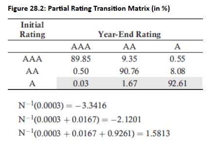
• Example: With an equity correlation of 0.2, correlated standard normal variables (xA,xB)(x_A, x_B)(xA​,xB​) are simulated to illustrate the probability of a rating change for an A-rated company.

• Rating transition thresholds: For an A-rated company, a realization of xA<−3.3416x_A < -3.3416xA​<−3.3416 implies an upgrade to AAA, while values between $-3.3416$ and $-2.1201$ imply a transition to AA.

• Extension across ratings: The same threshold-based approach applies to B-rated companies, allowing comparisons of rating transitions across the full rating spectru

• Model comparison insight: Differences in predicted outcomes between CreditMetrics and CreditRisk+ under identical assumptions are primarily driven by differences in the assumed timing of losses.

Topic 5. Credit Spread Risk

• Credit VaR and spread risk: The value of credit-sensitive products depends on credit spreads, so Credit VaR requires modeling potential credit spread changes, often using historical simulation to compute a one-day 99% VaR and scaling it to longer horizons.

• Limitations of simple historical approaches: Assuming consistent credit spread changes across firms is problematic due to:

  • infrequent daily spread data

  • the implicit assumption of no defaults when using histories of surviving firms.

• CreditMetrics framework: CreditMetrics addresses these issues by using rating transition matrices derived from historical rating changes, combined with Monte Carlo simulation to model rating migrations or defaults and revalue portfolios based on rating-specific credit spreads.

• Modeling credit correlation: Credit correlation can be incorporated either through a Gaussian copula linking rating transitions across firms or by assuming highly correlated credit spread movements across rating categories.

Topic 5. Credit Spread Risk

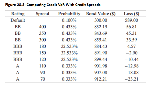
• Example: The firm holds a 3-year ZCB with face value $1,000; with a 2.5% risk-free rate and a 150 bp credit spread, the bond is priced at $1,000/(1.04)^3=$889. The bond is currently rated BBB.
  $1,000/(1.04)3=$889\$1{,}000 / (1.04)^3 = \$889

  • One-month rating scenarios and probabilities:

    • Upgrade to A: 1.0% probability; credit spreads = 70, 90, 110 bps (equally likely)

    • No change (BBB): 97.6% probability; credit spreads = 120, 150, 180 bps (equally likely)

    • Downgrade to BB: 1.3% probability; credit spreads = 300, 350, 400 bps (equally likely)

    • Default: 0.1% probability; bond value assumed to be $300

  • Valuation horizon: One month forward corresponds to 2.917 years remaining to maturity for the bond.

  • Credit VaR levels by confidence: The credit VaR is $589.00 at confidence levels above 99.9%, and $56.81 for confidence levels between 99.9% and 99.467%.

Topic 5. Credit Spread Risk

• Constant level of risk assumption: Credit VaR often assumes periodic rebalancing to maintain a constant risk profile, such as replacing downgraded bonds with bonds of the original rating (e.g., AA).

• Buy-and-hold vs constant risk: A buy-and-hold strategy typically results in larger losses from major downgrades and defaults, while small rating changes lead to lower loss probabilities.

• Impact on Credit VaR: Credit VaR is generally lower under a constant level of risk strategy than under a buy-and-hold strategy.

Practice Questions: Q3

Q3. When accounting for credit spreads and potential bond losses for a bond currently rated A, an analyst will likely assign the:

A. biggest spreads to situations where the bond rating increases.

B. lowest probability to situations where the bond rating increases.

C. lowest spreads to situations where the bond maintains its rating.

D. highest probability to situations where the bond maintains its rating.

Practice Questions: Q3 Answer

Explanation: D is correct.

An analyst will likely assign the highest probability to situations where the bond maintains its rating. The biggest spreads will be for situations where the bond rating decreases, and the lowest spreads will be for situations where the bond rating increases. The lowest probability will likely be for a bond default.