Book 5. Risk and Investment Management

FRM Part 2

IM 16. Liquidity Risk Management

Presented by: Sudhanshu

Module 1. Managing Fund Liquidity Risk

Module 2. Modeling Asset Liquidity

Module 3. Managing And Modeling Redemption Risk

Module 1. Managing Fund Liquidity Risk

Topic 1. Liquidity Risk Best Practices

Topic 2. Fixed-Income Liquidity Risk Challenges

Topic 1. Liquidity Risk Best Practices

• Definition and Context

  • Fund Liquidity Risk: The risk that a fund may be unable to obtain sufficient liquidity to meet investor redemptions, particularly complex for hedge funds due to asset types and the need to avoid disadvantaging remaining shareholders
  • Sources of Risk: Can arise from poor fund performance, reputational problems involving managers, or other operational issues

• Four Key Elements of Liquidity Risk Management Framework

  • Liquidity Risk Measurement: Risk managers identify, assess, and quantify key sources of liquidity risk
  • Liquidity Risk Management: Risk managers monitor the fund's liquidity profile and evaluate redemption risks against established limits
  • Portfolio Manager Liquidity Risk Awareness: Risk managers regularly review and discuss liquidity risks with portfolio managers, escalating material concerns to senior decision-makers (CRO or CIO) in a timely manner
  • Redemption Toolkit: Risk managers understand available backup liquidity tools and prepare to activate extraordinary measures when necessary

Topic 1. Liquidity Risk Best Practices

• Three Lines of Defense Models

  • First Line: Portfolio managers maintain consistent awareness of liquidity risk and hold primary responsibility for managing it
  • Second Line: Independent and robust risk management function provides oversight and control
  • Third Line: Periodic audits verify adherence to established policies by the first two lines of defense

• Liquidity Risk Management System Objectives and Key Variables

  • Comprehensive Measurement: System measures asset liquidity, analyzes redemption patterns, and ensures sufficient cash availability for expected redemptions
  • Fairness Goal: Avoid creating liquidity for departing investors in ways that leave remaining shareholders with an illiquid portfolio; balance redemption needs with preserving sound strategy for remaining investors
  • Influencing Variables: Market conditions (normal vs. stressed), position sizes, transaction costs, and potential market impact

Practice Questions: Q1

Q1. Within a robust liquidity risk management framework, which of the following situations most clearly indicates a governance or communication breakdown rather than a measurement or toolkit weakness?
A. The fund’s redemption toolkit includes swing pricing mechanisms for stressed markets.
B. Stress testing results trigger predefined limits and prompt partial portfolio rebalancing.
C. The risk function evaluates asset liquidity profiles under normal and stressed conditions.
D. Daily liquidity reports show tightening market depth, but no follow-up discussion occurs between risk management and portfolio management.

Practice Questions: Q1 Answer

Explanation: D is correct.

A failure to communicate or escalate known issues reflects a governance or communication breakdown. The other choices demonstrate effective measurement, management, or contingency-planning practices.

• Post-GFC Market Structure Changes

  • Corporate Borrowing Surge: Low interest rates after the 2007-2009 GFC encouraged significant corporate borrowing, including nonstandard issuances
  • Shift from Price Takers to Price Makers: Asset managers moved from accepting dealer quotes to setting their own transaction prices and seeking counterparties
    • Result: Thinner secondary markets with lower turnover and wider bid-ask spreads
    • Increased price impact of large transactions, leading managers to break trades into smaller orders
    • Liquidity costs rise with urgency and asset complexity (especially structured/specialized products)

• Price Discovery and Market Fragmentation

  • Equity vs. Fixed-Income Markets: Equity markets benefit from manageable security counts, frequent exchange trading, and strong price transparency; fixed-income markets are highly fragmented with limited price discovery
  • Scale of Fragmentation: Approximately one million municipal bond CUSIPs exist; only a small fraction of fixed-income securities trade on any given day, with activity concentrated in large, recently issued offerings
  • Valuation Complexity: Similar to valuing unique properties without perfect comparables, fixed-income valuation difficulty increases rapidly as product structure becomes more complex

Topic 2. Fixed-Income Liquidity Risk Challenges

• Data Availability Challenges

  • TRACE Reporting Limitations: FINRA's system provides daily price and volume data but caps reported trade volumes (high-yield >$1M, investment-grade >$5M shown only as "above cap")
  • Creates significant ambiguity whether actual volume is $6M or $60M
  • Models attempt to infer true volumes from historical patterns, risking inaccuracy when conditions change

• Recent Transparency Initiatives (As of 2025)

  • FINRA Enhancement: Provides uncapped trading volume at CUSIP level with six-month delay
  • MiFID II (Europe): Offers detailed intraday snapshots for liquid bonds; less liquid bond data released with one-month lag; requires asset managers to report realized transaction costs for European funds
  • Proposed EU Improvements: European Commission considering standardized consolidated tape—a unified data feed aggregating pricing and volume from all trading venues for equity and fixed-income securities

Topic 2. Fixed-Income Liquidity Risk Challenges

Practice Questions: Q2

Q2. Which of the following statements best explains why managing liquidity risk in fixed-income securities is often more difficult than in equity markets?
A. Fixed-income markets have fewer securities but trade more frequently with smaller bid-ask spreads.
B. Equity markets rely primarily on OTC transactions, reducing price transparency relative to fixed income.
C. Asset managers in fixed-income markets typically act as price takers, improving overall market liquidity.
D. Fixed-income markets contain a very large number of securities, many of which trade infrequently, making price discovery and valuation more difficult.

Practice Questions: Q2 Answer

Explanation: D is correct.

Fixed-income liquidity risk is harder to manage because the market is fragmented, securities trade infrequently, and price discovery is less reliable, especially compared with equities.

Module 2. Modeling Asset Liquidity

Topic 1. Days-to-Liquidate Approach

Topic 2. Modeling Liquidity for Infrequently Traded Bonds

Topic 3. Transaction Cost Modeling for Corporate Bonds

Topic 1. Days-to-Liquidate Approach

• Days-to-Liquidate Approach: Time required to unwind a specific investment position without causing significant market disruption.

• Components: The estimate is calculated based on three primary inputs:

  • ​Size of the Intended Trade: This can be determined by analyzing historical redemption patterns, portfolio leverage, and derivatives exposures.

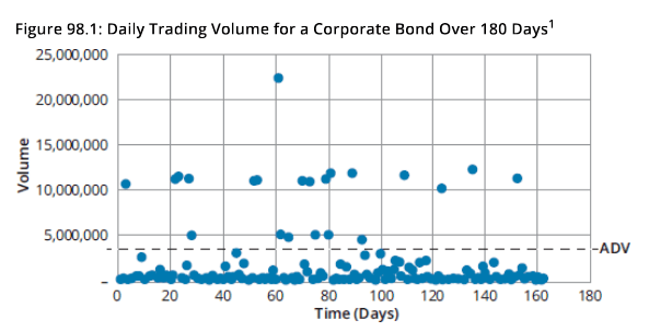
  • Assumed Market Participation Rate: Percentage of an asset's average daily volume (ADV) that can be sold without causing a material market impact. This rate is often difficult to estimate accurately.

    • ​In practice, actual trading volume is usually lower than the volume the market could theoretically support.

    • Latent Liquidity: Difference between observable liquidity and potential capacity.

  • ​Average Daily Volume (ADV): Average trading volume over a specific window, such as 20- or 60-day ADV.

    • Calculated using data from the firm, exchanges, or third-party vendors, and it can incorporate modeled inputs such as bonds outstanding or bid-ask spreads.

    • When direct data is limited, ADV can also be estimated using asset characteristics, sector-level turnover, or insights from experienced traders.

• Days-to-Liquidate Formula:

  • ​

  •  

Topic 2. Modeling Liquidity for Infrequently Traded Bonds

• Challenges: The infrequently trading makes it difficult to adapt the days-to-liquidate approach for infrequently traded bonds.

• Components of Infrequent Trading Problem

  • Estimating the probability that a trade will occur

  • Predicting the trade volume if the trade does occur

• Random Forest Regression Solution: Machine learning technique particularly suited for this application due to its ability to handle nonlinearity, missing data, and large sets of explanatory variables:

  •  

  • where:

    • b: The individual bond

    • t: current time

    •       : Bond b's trading volume at time t+1

    • TRADE: Condition for a trade to occur

    •       : Probability that Bond b trades at time t+1

    • E(V|TRADE): Expected trading volume specifically if a trade occurs

Topic 2. Modeling Liquidity for Infrequently Traded Bonds

• Historical Trading Activity: Reasonable guide for future volume when bonds trade frequently, but relationship breaks down for sporadically traded bonds; comparable bond data can help fill gaps for infrequent traders
• Dealer Inventory Information: Secondary market posted bids and asks help infer potential tradable volume
  • Actual trading volume typically lower than theoretical market capacity
  • Latent liquidity estimated using tail measures like 90th percentile of ADV distribution
• Volume Range Modeling: Framework quantifies security's potential liquidity within a range bounded by optimistic tail estimate and observed ADV
• Volume Variance Consideration: Large fluctuations in daily trading volume lead to significant variations in estimated volume; ADV can be conservative liquidity measure when volume variance is high

Practice Questions: Q1

Q1. Which of the following statements best describes a key challenge in modeling the liquidity risk of infrequently traded fixed-income securities using the days-to-liquidate approach?
A. Random forest regression cannot handle large feature sets or missing data.
B. Trade frequency and volume follow a linear pattern that basic regression can capture.
C. Bid prices perfectly represent true liquidity conditions, making volume variance irrelevant.
D. Relying on recent trade volumes can bias estimates because latent liquidity requires additional inference.

Practice Questions: Q1 Answer

Explanation: D is correct.

Latent liquidity and sparse trading activity mean that missing or incomplete data must be inferred, which introduces uncertainty into liquidity estimates for infrequently traded fixed-income securities.

Topic 3. Transaction Cost Modeling for Corporate Bonds

• T-Cost Fundamentals: Transaction costs are critical for assessing liquidity risk and best-execution verification; both liquidation time and potential market impact must be evaluated
• Liquidity Trade-offs: Rapid pro rata liquidation may cause adverse price effects, while maintaining higher ongoing liquidity can constrain return objectives
• Fixed-Income Pricing Challenges: Price is a primary input in t-cost modeling but carries significant uncertainty in fixed-income markets; recent standardization efforts aim to improve accuracy
• T-Cost Components:
  • Fixed costs: commissions and bid-ask spreads (can be normalized by midprice of benchmark quotes, though comparability weakens for infrequently traded bonds)
  • Market impact costs: reflect how position size affects execution costs
• Price Data Quality: Improving quality and availability of price data is a key priority for fixed-income liquidity risk modeling; lack of transparent and timely pricing creates noisy estimates requiring measurement error consideration
• Implementation Shortfall: Measures the difference between executed price and benchmark price; heavily dependent on accurate price discovery, which is often limited in fixed-income markets

Topic 3. Transaction Cost Modeling for Corporate Bonds

• T-Cost Modeling Approach: Uses intraday benchmark prices, empirical transaction data, and bond-specific attributes to forecast costs; regression techniques estimate model components with standard functional form capturing fixed costs (first component) and market impact costs (second component)

  •  

  •  

  • where

    • ​         : regression coefficients

    • BAS: percentage bid-ask spread

    • D: spread duration of convexity

    • S: option-adjusted spread of security

    • ADV: average daily volume from most recent ADV model

    •   : parameter that controls for shape of market impact

Topic 3. Transaction Cost Modeling for Corporate Bonds

• ​Measuring Market Impact using Implementation Shortfall: The primary purpose of t-cost modeling is to estimate market impact, which is measured through implementation shortfall.

• Implementation Shortfall: Difference between the traded price (the actual execution price) and the order-arrival benchmark price or another appropriate pre-trade benchmark.
  •  
  •  
  • where
    • sign = " 1 " for a buy order and " -1 " for a sell order
    • benchmark price = nearest intraday midprice at least five minutes before the trade
• Benchmark Selection for Implementation Shortfall
  • Previous end-of-day price as benchmark introduces significant return component, as market movements between yesterday's close and execution time are captured as costs
  • Intraday pre-trade benchmark price is considered best practice, better reflecting prevailing market conditions and less susceptible to manipulation

Topic 3. Transaction Cost Modeling for Corporate Bonds

• Regression-Based Transaction Cost Estimation:
  • Weight observations by dollar amount traded to account for the large number of small, odd-lot trades
  • Security-level data provides the most accurate insight for cost estimation
• Handling Limited Data with Cohorts:
  • When bond data is limited or missing, rely on cohorts of similar securities constructed using characteristics such as option-adjusted spread, duration, yield, or bid-ask spread
  • Machine learning techniques (clustering methods, tree-based models, neural networks) can identify degree of similarity across securities and improve estimate robustness

Practice Questions: Q2

Q2. When estimating transaction costs using t-cost modeling, why is an intraday, pre-trade benchmark price typically preferred over the previous end-of-day price? The intraday, pre-trade benchmark price:
A. reduces benchmark-related noise.
B. ensures that market impact is zero.
C. allows bid-ask spreads to be ignored.
D. eliminates the need to measure implementation shortfall.

Practice Questions: Q2 Answer

Explanation: A is correct.

Using the previous end-of-day price as the benchmark may introduce a large return component due to the long time gap between that price and the actual execution. Intraday, pre-trade benchmark prices better reflect current market conditions and reduce benchmark-related noise in the implementation shortfall used within the t-cost model.

Module 3. Managing And Modeling Redemption Risk

Topic 1. Meeting Unanticipated Redemption Requests

Topic 2. Modeling Redemption-at-Risk

Topic 3. Liquidity Optimization to Meet Redemption Requests

Topic 1. Meeting Unanticipated Redemption Requests

• Drivers of Redemption Pressure

  • Unexpected Outflow Triggers: Macroeconomic developments, poor fund performance, deterioration in manager reputation, severe peer fund underperformance (creating contagion risk), or fund-specific factors like investor profiles and concentration levels
  • Market Condition Impact: Redemption demand typically low under normal conditions before strategy maturity, but stressed markets can produce large, highly correlated redemption requests
  • Fair Treatment Objective: Manage redemptions equitably across three investor categories—those redeeming, those subscribing, and those remaining in the fund

Topic 1. Meeting Unanticipated Redemption Requests

• U.S. 40 Redemption Waterfall Structure

  • Layer 1 - Cash and Highly Liquid Assets:
    • Meet routine or unplanned redemption requests while minimizing transaction costs
    • Support derivatives overlay strategies for return enhancement
    • Respond strategically to market conditions
  • Layer 2 - Pro Rata or Risk-Constant Asset Sales: When Layer 1 assets are insufficient, sell less liquid holdings while ensuring remaining portfolio maintains approximately the same risk profile as before redemptions
  • Layer 3 - Short-Term Borrowings: Final option using backup liquidity sources such as reverse repos, overdraft facilities, or lines of credit; '40 Act funds limited to borrowing maximum 33.3% of total fund assets

• Stress Testing Framework

  • Scenario Application: Apply stress scenarios to fund assets, redemption volumes, average daily volume (ADV) assumptions, and transaction costs
  • Additional Considerations: Evaluate investor concentration, relevant historical redemption events, and potential effects of any gates in place

Practice Questions: Q1

Q1.  A U.S.-based hedge fund needs to use an extraordinary liquidity measure to meet unexpected redemption requests. Which of the following options is available to them?
A. Gates.
B. Suspension.
C. Swing pricing.
D. Temporary borrowing.

Practice Questions: Q1 Answer

Explanation: D is correct.

A U.S.-based hedge fund may use temporary borrowing (and in some cases, in-kind redemptions). They do not have access to gates, swing pricing, price mechanisms, or suspensions, which are options primarily available under European regulations such as UCITS.

Topic 2. Modeling Redemption-at-Risk

• Historical Redemption-at-Risk (HRAR): HRAR estimates worst-case outflows based on historical fund flows, such as 99th-percentile, five-day redemption scenarios over the fund's lifetime, providing potential stress signals for fund managers

• Key Modeling Challenges:
  • New or rapidly growing funds lack meaningful historical outflow data
  • Idiosyncratic investor behavior cannot be reliably modeled
  • Limited granular visibility when third-party custodians operate between funds and end investors
• Drivers of Large Outflows: Combination of systemic factors (sector-wide disruptions, macroeconomic shocks) and idiosyncratic factors (investor behavior, peer fund performance, cash flow needs, event-driven risks like scandals or regulatory sanctions)
• Machine Learning Applications: Can handle numerous redemption-influencing factors and capture nonlinear data relationships to estimate upper bounds on likely redemptions; however, implementation faces significant obstacles from data availability and quality limitations

Practice Questions: Q2

Q2. An analyst is applying the historical redemption-at-risk (HRaR) model to estimate potential redemption demand. Which of the following statements is least likely to represent a key challenge of this approach?
A. Some funds may lack sufficient redemption history because they are new or have been growing rapidly.
B. Limited transparency between asset managers and end investors can reduce the quality of available data.
C. Investor withdrawal behavior may be driven by idiosyncratic factors that are difficult to model statistically.
D. Historical data provides a stable and reliable indicator of future redemption pressures across all market environments.

Practice Questions: Q2 Answer

Explanation: D is correct.

Historical data is not a reliable predictor of future redemption stress, especially during market dislocations. The actual challenges include the absence of historical outflows for new or fast-growing funds, the influence of idiosyncratic investor behavior, and limited visibility into end investor activity when intermediaries operate between the fund and the investor.

Topic 3. Liquidity Optimization to Meet Redemption Requests

• Fund liquidity management can also be framed as an optimization problem in which managers balance liquidity, transaction costs, and portfolio risk while meeting redemption obligations.

• Layered Optimization Approach: Consider a layered approach to optimization using securities     with market value       and notional value

  • The portfolio manager must sell a pro rata fraction       of the portfolio on a given day t.

  • The first step is to determine the optimal pro rata fraction:

  • ​Objective Function: The goal is to maximize the liquidated market value while adhering to specific constraints:

    •  

    •  

• Actual or expected redemption obligations can be incorporated as constraints.

  • Example: The optimization of this expression could be constrained by a required liquidation amount v over a specified period, such as $200 million within two days. Adding such constraints enables a more detailed and cost-efficient design of the liquidation schedule.

Topic 4. Liquidity Optimization to Meet Redemption Requests

• ADV: To prevent excessive market impact, sales are limited by the security's ADV (    ) and an assigned participation rate (    ) for its sector j:

  • ​

• Market Capacity (     ): This accounts for the market's total ability to absorb supply in a specific sector (    ). This is critical because simultaneous large-scale sales of similar fixed-income securities can exhaust sector liquidity:

  • ​

  •  

• Time-Lag Constraints (    ): Certain assets, such as those with IPO lockups, cannot be sold before a specific date. In such cases, the fraction sold must be 0 until the lag period expires

  •  

• Risk Constraints (R): The manager must ensure the remaining portfolio stays below a specified risk threshold, such as a tracking error limit for index funds. The model uses the following summation to control for variance and covariance relative to a benchmark b:

  •  

  •  

• Note that the benchmark level     will equal zero for absolute return funds.

Topic 4. Liquidity Optimization to Meet Redemption Requests

• It should also be noted that the previous summation equation should include the full set of securities in both the benchmark and the portfolio. 

  • Additional optimization constraints may be incorporated as needed, including those related to cash use, tracking error, leverage limits, compliance requirements, and other fund-specific considerations.

• Summary of Implementation: The overall optimization process for meeting redemption requests is ultimately constrained by the quality and availability of the model’s input data.