Book 5. Risk and Investment Management
FRM Part 2
IM 6. VaR and Risk Budgeting in Investment Management
Presented by: Sudhanshu
Module 1. Budgeting and Managing Risk with VaR
Module 2. Monitoring Risk with VaR
Module 1. Budgeting and Managing Risk with VaR

Topic 1. Risk Budgeting
Topic 2. Managing Risk With VaR
Topic 3. Investment Process
Topic 4. Hedge Fund Issues
Topic 5. Absolute Risk vs. Relative Risk and Policy Mix vs. Active Risk
Topic 6. Funding Risk
Topic 7. Example: Determining a Fund's Risk Profile
Topic 8. Example: Surplus at Risk (by computing Volatility of Surplus)
Topic 9. Plan Sponsor Risk
Topic 1. Risk Budgeting
-
Definition: A top-down process of choosing and managing exposures to risk.
-
Main Idea: Risk manager establishes a total portfolio risk budget and allocates risk to individual positions based on a predetermined fund risk level.
-
Distinction: Differs from market value allocation as it focuses on the allocation of risk, not just capital.
Topic 2. Managing Risk With VaR
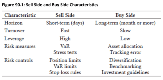
- The sell side (banks) developed VaR techniques years ago and have extensively used them, while the buy side (investors) are now adopting VaR but must adapt the techniques to fit their different business characteristics.
- Banks trade rapidly and cannot rely on traditional historical risk measures, as yesterday's risk may be irrelevant to today's positions, whereas investors typically hold positions for longer periods (e.g., years).
- VaR's dynamic risk measurement is critical for banks due to their high leverage, while institutional investors face stronger leverage constraints and have lower needs to control downside risk.
Practice Questions: Q1
Q1. With respect to the buy side and sell side of the investment industry, the:
I. buy side uses more leverage.
II. sell side has relied more on VaR measures.
A. I only.
B. II only.
C. Both I and II.
D. Neither I nor II.
Practice Questions: Q1 Answer
Explanation: B is correct.
Compared to banks on the “sell side,” investors on the “buy side” have a longer horizon, slower turnover, and lower leverage. Banks use forward-looking VaR risk measures and VaR limits.
Topic 3. Investment Process
-
Step 1: Determine long-term strategic asset allocations by balancing returns and risks using methods like mean-variance portfolio optimization across asset classes including domestic and foreign stocks, bonds, and alternative investments such as real estate, venture capital, and hedge funds.
- Strategic allocation relies on passive indices and benchmarks to measure investment properties and ensure allocations are feasible.
-
Step 2: Select managers who either passively track benchmarks or actively manage funds to outperform benchmarks, with periodic reviews of their activities and performance.
- Manager activities must conform to guidelines specifying investment types and risk exposure restrictions such as beta and duration, with performance evaluated through tracking error analysis.
- VaR risk management systems are increasingly important due to investment globalization, increased complexity, and the dynamic nature of investment companies where multiple managers making changes within their constraints can create difficult-to-gauge collective risk.
- Historical risk measures alone are no longer adequate given globalization, complexity, and industry dynamics, increasing the need for VaR-based risk management.
Topic 4. Hedge Fund Issues
-
Heterogeneous Asset Class: Includes a variety of trading strategies.
-
Risk Characteristics: Often similar to the "sell side" due to leverage and high trading volume.
-
Specific Risks:
-
Liquidity Risk: Potential loss from quick liquidation, difficulty in valuing the fund, and underestimation of traditional risk measures due to low liquidity.
-
Low Transparency: Makes risk measurement difficult regarding both size and type of risk, complicating overall portfolio risk management.
-
Topic 5. Absolute Risk vs. Relative Risk and Policy Mix vs. Active Risk
-
Absolute (Asset) Risk: Refers to total possible losses over a horizon and measured by the return over the horizon.
-
Relative Risk:
-
Measured by excess return (dollar loss relative to a benchmark).
-
Shortfall: Difference between fund return and benchmark return in dollar terms.
-
VaR techniques can apply to tracking error (standard deviation of excess return) if excess return is normally distributed.
-
-
Policy-Mix Risk: Risk associated with the target policy (weights assigned to various funds/asset classes).
-
Active Management Risk: Risk from managers making decisions that deviate from designated weights. It is often small due to diversification effects across deviations and with policy mix VaR. Also, well-managed funds have low active management risk as it is low for each of the individual funds.
Practice Questions: Q2
Q2. Compared to policy risk, which of the following is not a reason that management risk is not much of a problem?
A. There will be diversification effects across the deviations.
B. Managers tend to make the same style shifts at the same time.
C. For well-managed funds, it is usually fairly small for each of the individual funds.
D. There can be diversification with the policy mix VaR to actually lower the total portfolio VaR.
Practice Questions: Q2 Answer
Explanation: B is correct.
If managers make the same style shifts, then that would actually increase
management risk. All the other reasons are valid.
Topic 6. Funding Risk
- Definition: The risk that the value of assets will not be sufficient to cover the liabilities of an investment company (e.g., pension payouts).
- Some investment companies have zero funding risk while defined pension plans have the highest funding risk.
-
The focus of analysis is surplus and change in surplus, defined as:
-
-
In managing funding risk, analysts typically transform the nominal return on surplus into a return on assets and break down the return into its component parts.
-
- Evaluating above expression requires assumptions about future uncertain liabilities, which for pension funds represent "accumulated benefit obligations"—the present value of pension benefits owed to employees and beneficiaries.
- Determining present value requires a discount rate typically tied to current market interest rate levels.
- An ironic aspect of funding risk is that when interest rates decline, assets like equities and bonds typically increase in value, but the present value of future obligations may increase even more, potentially worsening the funding position.
-
Surplus at Risk (SaR): Occurs when the surplus turns negative, requiring additional contributions.
-
Immunization: Attempting to make the duration of assets equal to that of liabilities to mitigate funding risk, though not always feasible or desirable.
\begin{aligned}
\mathrm{R}_{\text {surplus }} & =\frac{\Delta \text { surplus }}{\text { assets }}=\frac{\Delta \text { assets }}{\text { assets }}-\left(\frac{\Delta \text { liabilities }}{\text { liabilities }}\right)\left(\frac{\text { liabilities }}{\text { assets }}\right) \\
& =\mathrm{R}_{\text {asset }}-\mathrm{R}_{\text {liabilities }}\left(\frac{\text { liabilities }}{\text { assets }}\right)
\end{aligned}
\text { Surplus = assets - liabilities and } \Delta \text { surplus }=\Delta \text { assets }-\Delta \text { liabilities }
Topic 7. Example: Determining a Fund's Risk Profile
-
Example: The XYZ Retirement Fund has $200 million in assets and $180 million in liabilities. Assume that the expected return on the surplus, scaled by assets, is 4%. This means the surplus is expected to grow by $8 million over the first year. The volatility of the surplus is 10%. Using a z-score of 1.65, compute VaR and the associated deficit that would occur with the loss associated with the VaR.
-
Solution: First, we calculate the expected value of the surplus. The current surplus is $20 million (= $200 million – $180 million). It is expected to grow another $8 million to a value of $28 million. As for the VaR:
-
VaR = (1.65)(10%)($200 million) = $33 million
-
-
If this decline in value occurs, the deficit would be the difference between the VaR and the expected surplus value: $33 million − $28 million = $5 million.
Topic 8. Example: Surplus at Risk (by computing Volatility of Surplus)
-
Example: The XYZ Retirement Fund has $200 million in assets and $180 million in liabilities. Assume that the expected annual return on the assets is 4% and the expected annual growth of the liabilities is 3%. Also assume that the volatility of the asset return is 10% and the volatility of the liability growth is 7%. Compute 95%surplus at risk assuming the correlation between asset return and liability growth is 0.4.
-
Solution: First, compute the expected surplus growth: 200*(0.04) -180*(0.03) = $2.6 million
-
Next, compute the volatility of the surplus growth. The variance of assets minus liabilities [i.e., var(A − L)] = var(A) + var(L) – 2*cov(A,L), where covariance is equal to the standard deviation of assets times the standard deviation of liabilities times the correlation between the two. The asset and liability amounts will also need to be applied to this formula.
-
-
Thus, SaR can be calculated by incorporating the expected surplus growth and standard deviation of the growth: 95% SaR = 2.6 − 1.65*18.89 = $28.57 million
-
\begin{aligned}
\text { Variance }(A-L)&=200^2 \times 0.10^2+180^2 \times 0.07^2-2 \times 200 \times 180 \times 0.10 \times 0.07 \times 0.4\\
&=400+158.76-201.6=\$ 357.16 \text { million } \\
\text { Standard Deviation }&=\sqrt{357.16}=\$ 18.89
\end{aligned}
Topic 9. Plan Sponsor Risk
-
Extension of Surplus Risk: Relates to those ultimately responsible for the pension fund.
-
Key Measures:
-
Economic Risk: Variation in the total economic earnings of the plan sponsor, considering how the risks of various components relate to each other (e.g., correlations between surplus and operating profits).
-
Cash Flow Risk: Variation of contributions to the fund; ability to absorb fluctuations allows for a more volatile risk profile.
-
-
Overall Goal: From the sponsor's viewpoint, management should focus on the variation of the firm's economic value by integrating risks associated with asset and surplus movements with overall financial goals, aligning with enterprise-wide risk management principles.
Module 2. Monitoring Risk with VaR
Topic 1. Using VaR to Monitor Risk
Topic 2. VaR Applications
Topic 3. Budgeting Risk
Topic 4. Budgeting Risk Across Asset Classes: Part I
Topic 5. Budgeting Risk Across Asset Classes: Part II
Topic 6. Optimal Asset Allocation
Topic 1. Using VaR to Monitor Risk
-
Identifying "Rogue Traders": VaR helps detect unauthorized trades or deviations from guidelines, especially in large firms.
-
Monitoring Passively Managed Portfolios: Even passive portfolios require VaR monitoring as benchmark risk profiles change over time (e.g., S&P 500 exposure shifts).
-
Analyzing Actively Managed Portfolios: VaR helps identify reasons for risk changes. Three explanations for dramatic changes in risk are:
-
Manager exceeding risk budget (temporary market change, unintentional drift, unauthorized trades).
-
Managers taking similar style bets (e.g., all moving into long-term bonds due to interest rate forecasts).
-
Increased market volatility (requiring decisions to accept or reduce risk).
-
-
Reverse Engineering VaR: Using tools like component VaR and marginal VaR to understand how individual position changes affect the overall portfolio risk.
-
Challenges: Measuring risk for unique asset classes (real estate, hedge funds, venture capital) and limited information on certain investments (emerging markets and IPOs).
-
Global Custodians: Trend towards single custodians for consolidated risk picture and forward-looking measures. Large custodian banks such as Citibank and DB are providing risk management products.
-
Client Demand: Clients increasingly ask money managers about their risk management systems, making comprehensive VaR systems.
Practice Questions: Q1
Q1. Using VaR to monitor risk is important for a large firm with many types of managers because:
A. it can help catch rogue traders and it can detect changes in risk from changes in benchmark characteristics.
B. although it cannot help catch rogue traders, it can detect changes in risk from changes in benchmark characteristics.
C. although it cannot detect changes in risk from changes in benchmark characteristics, it can help detect rogue traders.
D. of no reason. VaR is not useful for monitoring risk in large firms.
Practice Questions: Q1 Answer
Explanation: A is correct.
Both of these are reasons large firms find VaR and risk monitoring useful.
Topic 2. VaR Applications: Investment Guidelines
-
VaR helps move away from ad hoc procedures and overemphasis on notionals and sensitivities that characterize many current manager guidelines, as formal guidelines using established principles are superior to ad hoc approaches.
-
Limits on notionals and sensitivities are insufficient when leverage and derivatives positions exist, as they fail to account for variations in risk and correlations, whereas VaR limits incorporate all these factors.
-
Controlling positions rather than risk results in numerous rules and restrictions that may not achieve the main goal of measuring possible losses over a given time period—essential information for determining capital needed to meet liquidity needs.
-
Simple position restrictions can be easily evaded using the wide array of instruments now available, and as product ranges expand, traditional position-by-position guidelines become increasingly ineffective and cumbersome.
Topic 2. VaR Applications: Investment Process
- VaR aids the strategic asset allocation decision in the first step of the investment process by complementing mean-variance analysis and measuring specific risk changes when managers subjectively adjust weights from pure quantitative recommendations.
- At the trading level, VaR provides specific estimates of how a proposed position's risk affects the overall portfolio, beyond a trader's general intuition about return and standalone risk.
- An effective risk management system should automatically calculate marginal VaR for each existing and proposed position, enabling traders to choose positions with lower marginal VaR when faced with similar return characteristics.
- VaR methodology facilitates optimal portfolio construction by equalizing excess-return-to-marginal-VaR ratios across all asset types.
- Traders seeking the next best investment should focus on securities in asset classes with higher returns-to-marginal-VaR ratios to improve overall portfolio efficiency.
Practice Questions: Q2
Q2. VaR can be used to compose better guidelines for investment companies by:
I. relying less on notionals.
II. focusing more on overall risk.
A. I only.
B. II only.
C. Both I and II.
D. Neither I nor II.
Practice Questions: Q2 Answer
Explanation: C is correct.
Investment companies have been focusing on limits on notionals, which is cumbersome and has proved to be ineffective.
Topic 3. Budgeting Risk
-
Process: Determine total acceptable VaR for the firm and choose optimal asset allocation for that risk exposure. It is a top-down process.
-
Example Calculation (Firm Target): Firm with $100 million AUM, 20% return volatility target, 95% confidence level.
-
VaR = (1.65) * (20%) * ($100 million) = $33 million.
-
Goal: Choose assets for the fund that keep VaR less than this value
-
-
Portfolio Volatility Formula (for two assets W and X):
-
Where:
- weights of assets W and X
- volatilities of assets W and X
- correlation between assets W and X
- Diversification Effects: Sum of individual asset VaRs will be greater than actual portfolio VaR unless perfectly correlated. Risk budgeting must account for these diversification benefits across asset classes and down to individual assets.
-
Important Note: When calculating risk budgets for the exam, ignore expected returns if provided, as per the reading's conservative approach.
\sigma_{W+X}=\sqrt{\left(w_W^2 \sigma_W^2\right)+\left(w_X^2 \sigma_X^2\right)+\left(2 w_W w_X \rho_{W X} \sigma_W \sigma_X\right)}
w_W, w_X=
\sigma_W, \sigma_X=
\rho_{W X}=
Topic 4. Budgeting Risk Across Asset Classes: Part I
-
Example: A manager has a portfolio with only one position: a $500million investment in W. The manager is considering adding a $500million position X or Y to the portfolio. The current volatility of W is 10%. The manager wants to limit portfolio VaR to $200million at the 99% confidence level. Position X has a return volatility of 9% and a correlation withW equal to 0.7. Position Y has a return volatility of 12% and a correlation withW equal to zero. Determine which of the two proposed additions, X or Y, will keep the manager within his risk budget.
-
Answer: Currently, the VaR of the portfolio with only W is:
-
-
When adding X, the return volatility of the portfolio will be:
-
-
When adding Y, the return volatility of the portfolio will be:
- Thus, Y keeps the total portfolio within the risk budget.
\begin{aligned}
8.76 \%&=\sqrt{\left(0.5^2\right)(10 \%)^2+\left(0.5^2\right)(9 \%)^2+(2)(0.5)(0.5)(0.7)(10 \%)(9 \%)} \\
\operatorname{VaR}_{W+X}&=2.33(8.76 \%)(\$ 1,000 \text { million })=\$ 204 \text { million }
\end{aligned}
\mathrm{VaR}_{\mathrm{W}}=(2.33)(10 \%)(\$ 500 \text { million })=\$ 116.5 \text { million }
\begin{aligned}
7.81 \%&=\sqrt{\left(0.5^2\right)(10 \%)^2+\left(0.5^2\right)(12 \%)^2} \\
\operatorname{VaR}_{\mathrm{W}+\mathrm{Y}}&=(2.33)(7.81 \%)(\$ 1,000 \text { million })=\$ 182 \text { million }
\end{aligned}
Topic 5. Budgeting Risk Across Asset Classes: Part II
-
Example: Using the information provided in the previous example, demonstrate why focusing on the stand-alone VaR of X and Y would have led to the wrong choice.
-
Answer: Obviously, the VaR of X is less than that of Y.
- The individual VaRs would have led the manager to select X over Y; however, the high correlation of X withW gives X a higher incremental VaR, which puts the portfolio of W and X over the limit. The zero correlation ofW and Y makes the incremental VaR of Y much lower, and the portfolio ofW with Y keeps the risk within the limit.
\begin{aligned}
\operatorname{VaR}_X & =(2.33)(9 \%)(\$ 500 \text { million })=\$ 104.9 \text { million } \\
\operatorname{VaR}_Y & =(2.33)(12 \%)(\$ 500 \text { million })=\$ 139.8 \text { million }
\end{aligned}
Topic 6. Optimal Asset Allocation
-
The traditional method for evaluating active managers uses the information ratio, calculated as excess return (active return minus benchmark return) divided by tracking error.
-
-
-
-
For a portfolio of funds with separate managers, top management focuses on the portfolio information ratio across all funds.
-
-
If managers' excess returns are independent, optimal allocation weights are determined by the below formula that distributes capital across managers.
-
One way to use this measure is to “budget” portfolio tracking error.
- Given the , the , and the manager’s tracking error, top management can calculate the respective weights to assign to each manager.
-
The weights of the allocations to the managers do not necessarily have to sum to one.
-
Any difference can be allocated to the benchmark itself because, by definition, = 0.
-
Determining precise weights requires an iterative process, as each weight selection produces different portfolio expected excess returns and tracking errors.
\mathrm{IR}_{\mathrm{P}}=\frac{\text { (expected excess return of the portfolio) }}{\text { (the portfolio's tracking error) }}
\text { weight of portfolio managed by manager } i=\frac{\mathrm{IR}_{\mathrm{i}} \times \text { (portfolio's tracking error) }}{\mathrm{IR}_{\mathrm{p}} \times \text { (manager's tracking error) }}
\mathrm{IR}_{\mathrm{i}}=\frac{\text { (expected excess return of the manager) }}{\text { (the manager's tracking error) }}
\mathrm{IR}_{\mathrm{P}}
\mathrm{IR}_{\mathrm{i}}
\mathrm{IR}_{\mathrm{benchmark}}
Topic 6. Optimal Asset Allocation
-
Figure 90.2 illustrates a set of weights derived from the given inputs that satisfy the condition.
-
-
-
-
-
- From these calculations, we can observe that:
-
The conditions for optimal allocation hold true.
-
The difference between 100% and the sum of the weights 51% and 37% is the 12% invested in the benchmark.
-
\text { weight of portfolio managed by manager } A=\frac{\mathrm{IR}_{\mathrm{A}} \times \text { (portfolio's tracking error) }}{\mathrm{IR}_{\mathrm{p}} \times \text { (manager A's tracking error) }} =\frac{(3 \%)(0.70)}{(5 \%)(0.82)} = 51\%
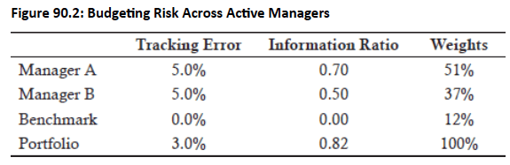
\text { weight of portfolio managed by manager } B=\frac{\mathrm{IR}_{\mathrm{B}} \times \text { (portfolio's tracking error) }}{\mathrm{IR}_{\mathrm{p}} \times \text { (manager B's tracking error) }} =\frac{(3 \%)(0.50)}{(5 \%)(0.82)} = 37\%
Practice Questions: Q3
Q3. In making allocations across active managers, which of the following represents the formula that gives the optimal weight to allocate to a manager denoted i, where and are the information ratios of the manager and the total portfolio, respectively?
A.
B.
C.
D.
\mathrm{IR}_i
\mathrm{IR}_p
\frac{\mathrm{I} \mathrm{R}_{\mathrm{p}} \times \text { (portfolio's tracking error) }}{\mathrm{I} \mathrm{R}_{\mathrm{i}} \times \text { (manager's tracking error) }}
\frac{\mathrm{IR}_{\mathrm{i}} \times \text { (manager's tracking error) }}{\mathrm{IR}_{\mathrm{0}} \times \text { (portfolio's tracking error) }}
\frac{\mathrm{IR}_{\mathrm{i}} \times \text { (portfolio's tracking error) }}{\mathrm{IR}_{\mathrm{p}} \times(\text { manager's tracking error })}
\frac{\mathrm{IR}_{\mathrm{p}} \times \text { (manager's tracking error) }}{\mathrm{IR}_{\mathrm{i}} \times \text { (portfolio's tracking error) }}
Practice Questions: Q3 Answer
Explanation: C is correct.
\text {Manager}_i=\frac{\mathrm{IR}_{\mathrm{i}} \times \text { (portfolio's tracking error) }}{\mathrm{IR}_{\mathrm{P}} \times \text { (manager's tracking error) }}
Copy of IM 6. VaR and Risk Budgeting in Investment Management
By Prateek Yadav


