Book 5. Risk and Investment Management

FRM Part 2

IM 7. Portfolio Performance Evaluation

Presented by: Sudhanshu

Module 1. Time-Weighted and Dollar-Weighted Returns

Module 2. Risk-Adjusted Performance Measures

Module 3. Alpha, Hedge Funds, Dynamic Risk, Market Risk and Style

Module 1. Time-Weighted and Dollar-Weighted Returns

Topic 1. Time-Weighted Returns 

Topic 2. Dollar-Weighted Returns

Topic 3. Dollar-Weighted Vs Time-Weighted Returns

Topic 1. Dollar-Weighted Returns

• Definition: The dollar-weighted rate of return is the Internal Rate of Return (IRR) on a portfolio.

• It accounts for the timing and size of all cash flows (inflows and outflows).

• Key Concept: It gives more weight to periods where larger sums of money are invested.

• Appropriate Use: Best for evaluating the performance of an investor who has control over the timing of their deposits and withdrawals. It reflects the return on the investor's actual invested capital.

• Calculating the Dollar-Weighted Rate of Return (Example)
• Scenario:

  • t = 0: Buy 1 share for $100.

  • t = 1: Buy 1 more share for $120. (Received a $2 dividend from the first share).

  • t = 2: Sell both shares for $130 each. (Received a $2 dividend per share).

• Cash Flows:

  • CF0​: -$100 (Initial Outlay)

  • CF1​: $2 (Dividend) - $120 (Purchase) = -$118

  • CF2​: ($130 * 2) (Sale Proceeds) + ($2 * 2) (Dividends) = +$264

• Formula: Set the present value of inflows equal to the present value of outflows and solve for $r$:

• Result: The IRR, or DWRR, is 13.86%.
• Time-Weighted Rate of Return (TWRR)

  • Definition: The time-weighted rate of return measures compound growth. It is the geometric mean of the holding period returns (HPRs) for each subperiod.

  • Key Concept: It completely removes the effect of cash inflows and outflows.

  • Appropriate Use: This is the preferred method for evaluating a portfolio manager's skill because their performance should not be judged by cash flow decisions made by the client, which are outside of their control.

Topic 1. Dollar-Weighted Returns

Practice Questions: Q1

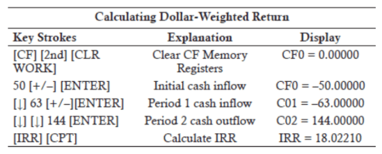
Q1. Assume you purchase a share of stock for $ 50 at time t=0 and another share at $ 65 at time t=1, and at the end of Year 1 and Year 2, the stock paid a $ 2.00 dividend. Also at the end of Year 2, you sold both shares for $ 70 each. The dollar-weighted rate of return on the investment is:

A. 10.77 %.

B. 15.45 %.

C. 15.79 %.

D. 18.02 %.

Practice Questions: Q1 Answer

Explanation: D is correct.

One way to do this problem is to set up the cash flows so that the PV of inflows = PV of outflows and then to plug in each of the multiple choices.

Alternatively, on your financial calculator, solve for IRR:

• Definition: The time-weighted rate of return measures compound growth. It is the geometric mean of the holding period returns (HPRs) for each subperiod.
• Key Concept: It completely removes the effect of cash inflows and outflows
• Appropriate Use: This is the preferred method for evaluating a portfolio manager's skill because their performance should not be judged by cash flow decisions made by the client, which are outside of their control.

Topic 2. Time-Weighted Returns

• Example: Calculating the Time-Weighted Rate of Return
  • Scenario: Same as the DWRR example.
• Calculation:

  • Step 1: Break the investment period into subperiods based on cash flows.

    • Subperiod 1: From t=0 to t=1.

    • Subperiod 2: From t=1 to t=2.

  • Step 2: Calculate the Holding Period Return (HPR) for each subperiod.

    •  

    •  

    •  

  • Step 3: Calculate the geometric mean of the HPRs.

    • ​

    •  

Topic 2. Time-Weighted Returns

Practice Questions: Q2

Q2.Assume you purchase a share of stock for $ 50 at time t=0 and another share at $ 65 at time t=1, and at the end of Year 1 and Year 2, the stock paid a $ 2.00 dividend. Also at the end of Year 2, you sold both shares for $ 70 each. The time-weighted rate of return on the investment is:

A. 18.04 %.

B. 18.27 %.

C. 20.13 %.

D. 21.83 %.

Practice Questions: Q2 Answer

Explanation: D is correct.

• Dollar-weighted returns are depressed when funds are contributed before poor performance periods and elevated when contributed before favorable periods, distorting manager ability assessment.
• Time-weighted returns remove these distortions and provide a better measure of a manager's investment selection ability over the period.
• Dollar-weighted returns may be more appropriate for private investors with complete control over account cash flows.
• Dollar-weighted returns will exceed time-weighted returns for managers with superior market timing ability.

Topic 3. Dollar-Weighted Vs Time-Weighted Returns

Module 2. Risk-Adjusted Perfomance Measures

Topic 1. Universe Comparisons

Topic 2. Sharpe Ratio

Topic 3. Treynor Measure

Topic 4. Jensen's Alpha

Topic 5. Information Ratio

Topic 6. M-Squared (M²) Measure: Overview

Topic 7. M-Squared (M²) Measure: Example

Topic 1. Universe Comparisons

• Concept: A method for comparing portfolios by first grouping them into categories based on their investment style (e.g., small-cap growth, large-cap value) and then ranking them based on their return within their specific style universe.

• Purpose: This approach makes rankings more meaningful by standardizing the comparison based on investment style.

• Limitation: It may not fully account for all risk differences if there is still variation in risk profiles among the funds within a single style.

Topic 2. The Sharpe Ratio

• Definition: Measures the amount of excess return (above the risk-free rate) earned per unit of total risk.

• Formula: 

  
  ​​

• Variables:

  •       Sharpe Ratio

  •     ​ : Average account return   

  • ​    : Average risk-free return

  •     : Standard deviation of account returns (total risk)

• Key Insight: The Sharpe Ratio evaluates a portfolio's performance in terms of both overall return and diversification, as it uses total risk as the denominator.

Topic 3. The Treynor Measure

• Definition: Similar to the Sharpe Ratio, but measures the excess return per unit of systematic risk (beta).

• Formula: 

  
  ​​

• Variables:

  • ​    : Treynor Measure

  •       ​ : Average account return

  •        ​: Average risk-free return

  •     : Average beta (systematic risk)

• For a well-diversified portfolio,

  • The Sharpe and Treynor rankings will be similar.

  • A higher Treynor ranking compared to the Sharpe ranking suggests the presence of significant unsystematic risk.

Practice Questions: Q1

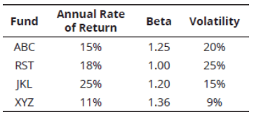
Q1. The following information is available for Funds ABC, RST, JKL, and XYZ:

The average risk-free rate was 5%. Rank the funds from best to worst according to their Treynor measure.

A. JKL, RST, ABC, XYZ.

B. JKL, RST, XYZ, ABC.

C. RST, JKL, ABC, XYZ.

D. XYZ, ABC, RST, JKL.

Practice Questions: Q1 Answer

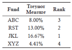
Explanation: A is correct.

Treynor measures:

The following table summarizes the results:
 

Topic 4. Jensen's Alpha

• Definition: The difference between a portfolio's actual return and its expected return, as predicted by the Capital Asset Pricing Model (CAPM). It is a direct measure of a manager's performance.

• Formula: 

  αA​=RA​−E(RA​)

  where:

  E(RA​)=RF​+βA​[E(RM​)−RF​]

• Variables:

  • αA​: Jensen's Alpha

  • RA​: Actual return on the account

  • E(RA​): Expected return based on CAPM

  • RF​: Risk-free rate

  • E(RM​): Expected market return

  • βA​: Average beta

• Key Insight: A positive and statistically significant alpha indicates a superior manager who has outperformed the market on a risk-adjusted basis. Like the Treynor measure, it only considers systematic risk.

Practice Questions: Q2

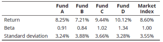
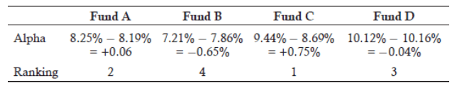
Q2. The following data has been collected to appraise Funds A, B, C, and D:

The risk-free rate of return for the relevant period was 4%. Calculate and rank the funds from best to worst using Jensen’s alpha.

A. B, D, A, C.

B. A, C, D, B.

C. C, A, D, B.

D. C, D, A, B.

Practice Questions: Q2 Answer

Explanation: C is correct.

CAPM returns:

Topic 5. The Information Ratio

• Definition: Measures a portfolio's surplus return relative to a benchmark, divided by the standard deviation of that surplus return.

• Formula: 

  
  ​

• Variables:

  • IRA​: Information Ratio

  •        : Average account return

  •             ​: Average benchmark return

  • σA−B​: Standard deviation of the excess returns (difference between account and benchmark returns)

• Key Insight: A higher Information Ratio indicates better performance, as it shows the amount of "risk" (variability of surplus returns) taken to achieve returns above the benchmark.

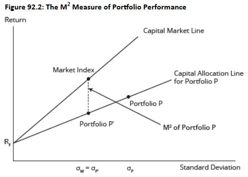
Topic 6. The M-Squared (M²) Measure: Overview

• Definition: The M² measure compares the managed portfolio's return against the market return after adjusting for differences in total risk (standard deviation).

• Concept: The M² measure can be illustrated with a graph comparing the capital market line for the market index and the capital allocation line for managed Portfolio P.

  • A hypothetical portfolio (P’) is created by combining the managed portfolio ($P$) and a risk-free asset to match the standard deviation of the market portfolio.

• Calculation: The M² measure is the difference in returns between this hypothetical portfolio (P’) and the market portfolio.

• Key Insight: The M² measure will produce the same rankings as the Sharpe Ratio, as both are based on total risk.

Topic 6. The M-Squared (M²) Measure

• M² produces the same conclusions as the Sharpe ratio, and Jensen's alpha produces the same conclusions as the Treynor measure. 

• M² and Sharpe ratio may not give the same conclusion as Jensen's alpha and Treynor measure due to potential discrepancies. 

• A discrepancy occurs when a manager takes on a large proportion of unsystematic risk relative to systematic risk, which lowers the Sharpe ratio but leaves the Treynor measure unaffected. 

Topic 7. The M-Squared (M²) Measure: Example

• Calculate the M² performance measure based for Portfolio P based on given data as:

  • Portfolio P mean return = 10% and standard deviation =40%

  • Market portfolio mean return = 12%and standard deviation = 20%

  • Risk-free Rate = 4%

• ​First note that a portfolio, P’, can be created that allocates 50/50 to the risk-free asset and to Portfolio P such that:
  • ​

• The mean return on Portfolio P’:

  • ​

• Therefore, we now have created a portfolio, P’, that matches the risk of the market portfolio (standard deviation equals 20%).

• Now, we can  calculate the difference in returns between Portfolio P’ and the market portfolio:

  •  

• Clearly, Portfolio P is a poorly performing portfolio. After controlling for risk, Portfolio P provides a return that is 5 percentage points below the market portfolio.

Module 3. Alpha, Hedge Funds, Dynamic Risk, Market Timing and Style

Topic 1.  Statistical Significance of Alpha Returns

Topic 2. Measuring Hedge Fund Performance

Topic 3. Performance Evaluation With Dynamic Risk Levels

Topic 4. Measuring Market Timing with Regression

Topic 5. Measuring Market Timing with a Call Option Model

Topic 6. Sharpe's Style Analysis: Overview

Topic 7. Steps of Sharpe's Style Analysis

Topic 1. Statistical Significance of Alpha Returns

• To determine if a positive alpha is a result of a manager's skill or merely a random outcome, we conduct a t-test under the following  hypotheses.

  • ​Null (     ): True alpha is zero.

  • Alternative (      ): True alpha is not zero.

• The t-statistic is computed as:

  •  

  •  

  • where,

    •  

    •  

    •  

    •  

• Key Concept: A statistically significant alpha (indicated by a high t-statistic) suggests that the manager has indeed outperformed the market on a risk-adjusted basis. A positive alpha that is not statistically significant may just be due to luck.

Topic 2. Measuring Hedge Fund Performance

• Long-short hedge funds complement well-diversified portfolios by providing positive alpha with zero beta, creating portable alpha independent of broad market performance that can be added to any existing portfolio.
• The market-neutral structure allows alpha generation outside the investor's desired asset class mix.

• Hedge fund performance evaluation is complicated because:

  • Hedge fund risk is not constant over time (nonlinear risk).

  • Hedge fund holdings are often illiquid (data smoothing).

  • Hedge fund sensitivity with traditional markets increases in times of a market crisis and decreases in times of market strength.

• This problem necessitates the use of estimated prices for hedge fund holdings. Therefore, the values of the hedge funds are not transactions-based and are rather estimation-based.

• The estimation process unduly smooths the hedge fund “values,” inducing serial correlation into any statistical examination of the data.

Topic 3. Performance Evaluation With Dynamic Risk Levels

• Sharpe ratio works best for passive strategies with stable risk-return characteristics.

• For active strategies, where volatility and returns fluctuate, the ratio can give biased or misleading results.

• Example 1 (Low-risk year 1): Quarterly returns are −2%, 4%, −2%, and 4%

  • Alpha = 1%, σ = 3%, Sharpe = 0.3333, outperforming market Sharpe of 0.3

• Example 2 (High-risk year 2): Quarterly returns are −10%, 20%, −10%, and 20%

  • Alpha = 5%, σ = 15%, Sharpe = 0.3333, still above market Sharpe of 0.3

• Combining both years: Average excess return = 3%, σ = 11%, Sharpe = 0.2727 → below market Sharpe.

• The drop in Sharpe ratio occurs due to increased overall volatility from changing strategies.

• Key takeaway: Dynamic shifts in portfolio risk can distort Sharpe ratio comparisons and lead to incorrect performance rankings.

Topic 4. Measuring Market Timing with Regression

• Market timing models extend basic return regressions to test a manager’s ability to adjust portfolio beta based on market expectations.

• A skilled market timer increases beta in rising markets and decreases it in falling markets to outperform benchmarks.

• The regression model used is:

  • 
    RP−RF=α+β(RM−RF)+MP(RM−RF)D+ϵR_P - R_F = \alpha + \beta (R_M - R_F) + M_P (R_M - R_F)D + \epsilon

• D is a dummy variable:

  • 0 for down markets

  • 1 for up markets

• MP represents the difference between upmarket and downmarket betas:

  • Beta in bear market =

  • Beta in bull market =

• A positive MP indicates successful market timing ability.

• Empirical studies show that MP is often negative for most mutual funds, implying poor or nonexistent market timing skills among fund managers.

Topic 5. Measuring Market Timing with a Call Option Model

• Perfect foresight investor: Allocates 100% to:

  • S&P 500 when E(RM)>RFE(R_M) > R_FE(RM​)>RF​

  • Treasury bills when E(RM)<RFE(R_M) < R_FE(RM​)<RF​.

• Return outcomes:

  • RMR_MRM​ if RM>RFR_M > R_FRM​>RF​ (market outperforms)

  • RFR_FRF​  if RM<RFR_M < R_FRM​<RF​ (market underperforms).

• Replication strategy: invest S0S_0S0​ in Treasury bills and buy a call option on the S&P 500 with strike price S0(1+RF)S_0(1 + R_F)S0​(1+RF​).

• Up-market scenario:

  • Option payoff = S0[(1+RM)−(1+RF)]S_0[(1 + R_M) - (1 + R_F)]S0​[(1+RM​)−(1+RF​)]

  • Treasury bill FV offsets strike price → total = S0(1+RM)S_0(1 + R_M)S0​(1+RM​)

• Down-market scenario:

  • Call expires worthless; T-bills return RFR_FRF​.

• Result: The calls + bills portfolio replicates perfect foresight returns.

• Implication: The value of perfect market timing equals the price of a call option on the market index.

Topic 6. Sharpe's Style Analysis: Overview

• William Sharpe developed the concept of style analysis to decompose portfolio returns.

• Analyzed Fidelity’s Magellan Fund (1985–1989) to separate style (asset allocation) and selection (security choice/market timing) effects.

• Findings:

  • 97.3% of returns explained by style bets (asset allocation).

  • 2.7% attributed to selection bets (security selection and timing).

• Empirical evidence confirms that long-term asset allocation is the dominant driver of performance.

• Conclusion: Market timing and stock selection contribute minimally and often fail to justify their costs

Topic 7.  Steps of Sharpe's Style Analysis

• Step 1: Run a regression of portfolio returns against an exhaustive and mutually exclusive set of asset class indices:

  •  

  •  

  •  

  • Here, the slopes/weights are constrained to be ≥0 and to sum to 100%. In that manner, the slopes can be interpreted to be “effective” allocations of the portfolio across the asset classes.​​

• ​​Step 2:  Conduct a performance attribution (return attributable to asset allocation & to selection):
  • ​Performance %age attributable to asset allocation =     (the coefficient of determination).
  • Performance  %age attributable to selection =

  • The asset allocation attribution equals the difference in returns attributable to active asset allocation decisions of the portfolio manager:

  • The selection attribution equals the difference in returns attributable to superior individual security selection (correct selection of mispriced securities) and sector allocation (correct over and underweighting of sectors within asset classes):

  • Note that the combination of the two attribution components (asset allocation plus selection) equals the aggregate contribution:

Topic 7.  Steps of Sharpe's Style Analysis

• Step 3: Uncover the investment style of the portfolio manager: the regression slopes are used to infer the investment style of the manager. For example, assume the following results are derived:

  •  

  • where

    • ​

    •  

    •  

  • The regression results indicate that the manager is pursuing primarily a large-cap growth investment style.​​​

Practice Questions: Q1

Q1. Sharpe’s style analysis, used to evaluate an active portfolio manager’s performance, measures performance relative to:

A. a passive benchmark of the same style.

B. broad-based market indices.

C. the performance of an equity index fund.

D. an average of similar actively managed investment funds.

Practice Questions: Q1 Answer

Explanation: A is correct.

Sharpe’s style analysis measures performance relative to a passive benchmark of the same style.