Book 1. Market Risk
FRM Part 2
MR 12. Arbitrage Pricing with Term Structure Models
Presented by: Sudhanshu
Module 1. Interest-Rate Trees and Risk-Neutral Pricing
Module 2. Binomial Trees
Module 3. Option-Adjusted Spread
Module 1. Interest-Rate Trees and Risk-Neutral Pricing
Topic 1. Binomial Interest Rate Tree
Topic 2. Features of a Binomial Interest Rate Tree
Topic 3. Constructing the Binomial Interest Rate Tree
Topic 4. Valuing an Option-Free Bond Using Backward Induction
Topic 5. Risk-Neutral Pricing and Interest Rate Drift
Topic 6. Using the Risk-Neutral Interest Rate Tree

Topic 1. Binomial Interest Rate Tree
- The binomial interest rate model is used throughout this reading to illustrate the issues considered when valuing bonds with embedded options.
- Definition: A binomial model is one that assumes interest rates can take only one of two possible values in the next period.
- Assumptions: The binomial model makes assumptions about interest rate volatility and a set of paths that interest rates may follow over time. This set of possible interest rate paths is called an interest rate tree.
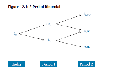
- A 2-period binomial tree is shown below.
-
A binomial interest rate tree is characterized by below features:
-
Node: A node is a point in time when interest rates can follow one of two possible paths: an upper path (U) or a lower path (L). The upper path from a given node leads to a higher rate than the lower path.
-
Rate Labeling (2-Period Example): The rate i2,LU is the rate that occurs if the initial rate i0 follows the lower path to period 1 (becoming i1,L) and then follows the upper path to period 2.
-
Recombining Tree: In a recombining tree, an upward move followed by a downward move gets to the same place as a down-then-up move, so i2,LU=i2,UL.
-
Rates in the Tree: The interest rates at each node in the tree are 1-period forward rates corresponding to the nodal period. Beyond the root, there is more than one 1-period forward rate for each nodal period (e.g., at Year 1, there are two 1-year forward rates, i1,U and i1,L).
-
Rate Relationship: The relationship among the rates associated with each individual nodal period depends on the interest rate volatility assumption of the model used to generate the tree.
-
Topic 2. Features of a Binomial Interest Rate Tree
Topic 3. Constructing the Binomial Interest Rate Tree
-
Underlying Rule: The values for on-the-run issues generated using an interest rate tree must prohibit arbitrage opportunities.
-
Arbitrage-Free Requirement: This means the value of an on-the-run issue produced by the interest rate tree must equal its market price.
-
Volatility Maintenance: The interest rate tree must maintain the interest rate volatility assumption of the underlying model.
-
Practical Construction: In practice, the interest rate tree is typically generated using specialized computer software.
Topic 4. Valuing an Option-Free Bond Using Backward Induction
-
Backward Induction: This term refers to the process of valuing a bond using a binomial interest rate tree.
-
Process: The current value of a bond with N compounding periods is determined by computing the bond's possible values at period N and working "backward" to node 0.
-
Value at a Node: The value of a bond at a given node in a binomial tree is the average of the present values of the two possible values from the next period.
-
Discount Rate: The appropriate discount rate is the forward rate associated with the node under analysis.
-
Coupon Bonds: When valuing bonds with coupon payments, the coupon should be added to the bond prices at each node before computing present values.
-
Arbitrage-Free Example: If the computed value of the bond at node 0 equals the market price, the binomial tree is considered arbitrage free.
-
For an option-free bond, the value (Vnode) is calculated as:
-
-
-
where Vup and Vdown are the values (including coupon, if any) at the next period's nodes, and rnode is the forward rate at the current node.
-
V_{\text{node}}=\frac{(V_{\text{up}} \times 0.5)+(V_{\text{down}}\times 0.5)}{1+r_{\text{node}}}
Topic 4. Valuing an Option-Free Bond Using Backward Induction
-
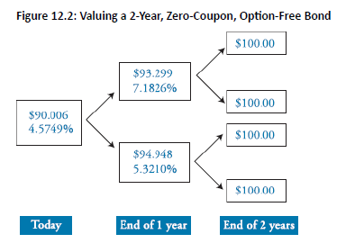
Example: Assuming the bond’s market price is $90.006, demonstrate that the tree in Figure 12.2 is arbitrage free using backward induction.
- Therefore,
-
Since the computed value of the bond equals the market price, the binomial tree is arbitrage free.
V_{\text{1,U}}=\frac{( \$100 \times 0.5)+( \$100 \times 0.5)}{1.071826}=\$93.299 \text{ and } V_{\text{1,L}}=\frac{( \$100 \times 0.5)+( \$100 \times 0.5)}{1.053210}=\$94.948
V_{\text{0}}=\frac{( \$93.299 \times 0.5)+( \$94.948 \times 0.5)}{1.045749}=\$90.006
Practice Questions: Q1
Q1. Which of the following statements concerning the calculation of value at a node in a fixed-income binomial interest rate tree is most accurate? The value at each node is the:
A. present value of the two possible values from the next period.
B. average of the present values of the two possible values from the next period.
C. sum of the present values of the two possible values from the next period.
D. average of the future values of the two possible values from the next period.
Practice Questions: Q1 Answer
Explanation: B is correct.
The value at any given node in a binomial tree is the average present value of the cash flows at the two possible states immediately to the right of the given node, discounted at the 1-period rate at the node under examination.
Topic 5. Risk-Neutral Pricing and Interest Rate Drift
- Using 0.5 probabilities for up and down movements in a binomial tree may not yield an expected discounted value equal to the bond's market price, since these represent the assumed true probabilities of price movements rather than risk-neutral probabilities.
- To align the binomial tree's discounted value with the actual market price, risk-neutral probabilities must be used instead of the true 0.5 probabilities.
- Risk-neutral probabilities are the adjusted probabilities that ensure the discounted expected value matches the current market price of the bond.
- The difference between risk-neutral probabilities and true probabilities is called the interest rate drift, which accounts for the market's risk preferences and ensures proper valuation.
Topic 6. Using the Risk-Neutral Interest Rate Tree
-
Risk-neutral pricing refers to the method used to compute bond and bond derivative values using a binomial model. There are two such methods:
-
Arbitrage-Free Tree (Adjust Rates)
-
Start with spot/forward rates from current yield curve
- Adjust interest rates on tree paths so model value equals market price of on-the-run bond
- Use derived interest rate tree to price derivatives by calculating expected discounted value at each node with real-world probabilities
-
-
Risk Neutral Probabilities (Adjust Probabilities)
- Take tree rates as given
- Adjust probabilities so model bond value equals current market price
- Price derivatives using expected discounted value at each node with risk-neutral probabilities, working backward through tree
-
- The value of the derivative is the same under either method.
Module 2. Binomial Trees
Topic 1. Valuing an Option on Fixed-Income Securities
Topic 2. Valuing a Callable Bond: Example
Topic 3. Recombining and Non-Recombining Trees
Topic 4. Constant-Maturity Treasury (CMT) Swap
Topic 1. Valuing an Option on Fixed-Income Securities
-
There are three basic steps to valuing an option on a fixed-income instrument using a binomial tree:
-
Step 1: Price the bond value at each node using the projected interest rates.
-
Step 2: Calculate the intrinsic value of the derivative at each node at maturity.
-
Step 3: Calculate the expected discounted value of the derivative at each node using the risk-neutral probabilities and working backward through the tree.
-
-
The option cannot be properly priced using expected discounted value because the call option value depends on the path of interest rates over the life of the option.
-
Incorporating the various interest rate paths will prohibit arbitrage from occurring.
Topic 2. Valuing a Callable Bond: Example
-
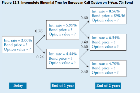
Consider a European call option with 2 years to expiration and a strike price of $100.00. The underlying is a 7%, annual coupon bond with 3 years to maturity. Figure 12.3 shows the first 2 years of the binomial tree for valuing the underlying bond. Assume that the risk-neutral probability of an up move is 0.76 in Year 1 and 0.60 in Year 2. Fill in the missing data in the binomial tree, and calculate the value of the European call option.
Topic 2. Valuing a Callable Bond: Solution (Step 1)
-
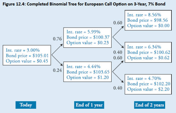
Step 1: Calculate the bond prices at each node using the backward induction methodology. Remember to add the 7% coupon payment to the bond price at each node when discounting prices. At the middle node in Year 2, the price is $100.62. You can calculate this by noting that at the end of Year 2 the bond has one year left to maturity:
-
N = 1; I/Y = 6.34; PMT = 7; FV = 100; CPT → PV = 100.62
-
-
At the bottom node in Year 2, the price is $102.20:
-
N = 1; I/Y = 4.70; PMT = 7; FV = 100; CPT → PV = 102.20
-
-
At the top node in Year 1, the price is $100.37:
-
At the bottom node in Year 1, the price is $103.65:
-
Today, the price is $105.01:
-
\frac{(\$ 105.56 \times 0.6)+(\$ 107.62 \times 0.4)}{1.0599}=\$ 100.37
\frac{(\$ 107.62 \times 0.6)+(\$ 109.20 \times 0.4)}{1.0444}=\$ 103.65
\frac{(\$ 107.37 \times 0.76)+(\$ 110.65 \times 0.24)}{1.03}=\$ 105.01
Topic 2. Valuing a Callable Bond: Solution (Steps 2 & 3)
-
Step 2: Determine the intrinsic value of the option at maturity in each node. For example, the intrinsic value of the option at the bottom node at the end of Year 2 is $2.20 = $102.20 − $100.00. At the top node in Year 2, the intrinsic value of the option is zero since the bond price is less than the call price.
-
Step 3: Using the backward induction methodology, calculate the option value at each node prior to expiration. For example, at the top node for Year 1, the option price is $0.23:
-
The option value today is:
- Fig 12.4 shows the complete tree.
\frac{(\$ 0.00 \times 0.6)+(\$ 0.62 \times 0.4)}{1.0599}=\$ 0.23
\frac{(\$ 0.23 \times 0.76)+(\$ 1.20 \times 0.24)}{1.03}=\$ 0.45
Practice Questions: Q1
Q1. A European put option has two years to expiration and a strike price of $101.00. The underlying is a 7% annual coupon bond with three years to maturity. Assume that the risk-neutral probability of an up move is 0.76 in Year 1 and 0.60 in Year 2. The current interest rate is 3.00%. At the end of Year 1, the rate will either be 5.99% or 4.44%. If the rate in Year 1 is 5.99%, it will either rise to 8.56% or rise to 6.34% in Year 2. If the rate in one year is 4.44%, it will either rise to 6.34% or rise to 4.70%. The value of the put option today is closest to:
A. $1.17.
B. $1.30.
C. $1.49.
D. $1.98.
Practice Questions: Q1 Answer
Explanation: A is correct.
This is the same underlying bond and interest rate tree as in the call option example from this reading. However, here we are valuing a put option. The option value in the upper node at the end of Year 1 is computed as:
The option value in the lower node at the end of Year 1 is computed as:
The option value today is computed as:
\frac{(\$ 2.44 \times 0.6)+(\$ 0.38 \times 0.4)}{1.0509}=\$ 1.52
\frac{(\$ 0.38 \times 0.6)+(\$ 0.00 \times 0.4)}{1.0444}=\$ 0.22
\frac{(\$ 1.52 \times 0.76)+(\$ 0.22 \times 0.24)}{1.0300}=\$ 1.17
Topic 3. Recombining and Non-Recombining Trees
-
A binomial tree can be described as either recombining or nonrecombining.
-
Recombining Tree:
-
In a recombining tree, the interest rate in a node of a later period is the same regardless of the path taken (e.g., up then down, or down then up).
-
The tree used in the call option example, where the interest rate at the middle node of period two was 6.34% for both paths, is a recombining tree.
-
-
Nonrecombining Tree:
-
A nonrecombining tree occurs when the up-then-down scenario produces a different interest rate than the down-then-up scenario.
-
This may result from state-dependent volatility, where the interest rate movement (e.g., a fixed number of basis points) depends on whether the current rate is above or below a certain level.
-
While nonrecombining trees may be more appropriate from an economic standpoint, prices can be very difficult to calculate when the binomial tree is extended to multiple periods.
-
-
Topic 4. Constant-Maturity Treasury (CMT) Swap
-
Definition: A swap where a floating rate is exchanged for a Treasury rate with a constant maturity (e.g., 10-year CMT).
-
Example: Assume that you want to value a CMT swap. The swap pays the following every six months until maturity:
-
is a semiannually compounded yield, of a predetermined maturity, at the time of payment, and is equivalent to 6-month spot rate. Assume there is a 76% risk- neutral probability of an increase in the 6-month spot rate and a 60% risk-neutral probability of an increase in the 1-year spot rate. Fill in the missing data in the binomial tree, and calculate the value of the swap.
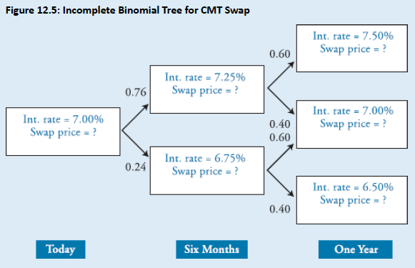
\left(\frac{\$ 1,000,000}{2}\right) \times\left(\mathrm{y}_{\mathrm{CMT}}-7 \%\right)
y_{CMT}
Topic 4. Constant-Maturity Treasury (CMT) Swap
-
In six months, the top node and bottom node payoffs are, respectively:
-
-
Similarly in one year, the top, middle, and bottom payoffs are, respectively:
-
-
Hence, the 6-month values for the top and bottom node are, respectively:
-
c
-
-
The price today is:
-
-
Fig 12.6 shows complete tree.
\text { payoff }{ }_{1, \mathrm{U}}=\frac{\$ 1,000,000}{2} \times(7.25 \%-7.00 \%)=\$ 1,250 \text{; } \text { payoff }_{1, L}=\frac{\$ 1,000,000}{2} \times(6.75 \%-7.00 \%)=-\$ 1,250
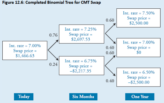
\mathrm{V}_0=\frac{(\$ 2,697.53 \times 0.76)+(-\$ 2,217.35 \times 0.24)}{(1+0.07/2)}=\$ 1,466.63
\text { payoff }_{2, \mathrm{U}}=\$2,500 \text{; } \text { payoff }_{2, \mathrm{M}}=\$0 \text{; } \text { payoff }_{2, \mathrm{L}}=-\$2,500
V_{1, U}=\frac{(\$ 2,500 \times 0.6)+(\$ 0 \times 0.4)}{(1+0.0725/2)}+\$ 1,250=\$ 2,697.53 \text{; } V_{1, L}=\frac{(\$ 0 \times 0.6)+(-\$ 2,500 \times 0.4)}{(1+0.0675/2)}-\$ 1,250=-\$ 2,217.35
Module 3. Option-Adjusted Spread
Topic 1. Option-Adjusted Spread (OAS)
Topic 2. Time Steps
Topic 3. Fixed-Income Securities and Black-Scholes-Merton (BSM) Model
Topic 4. Callable Bonds
Topic 5. Putable Bonds
Topic 1. Option-Adjusted Spread(OAS)
-
Definition: The OAS is the spread that makes the model value (calculated by the present value of projected cash flows) equal to the current market price.
-
Application to Pricing: When valuing a security with a binomial tree, the OAS is added to each discounted risk-neutral rate in the tree.
-
Impact on Discount Rates: The OAS only adjusts the rates used for discounting values. It does not impact the rates used for estimating cash flows.
-
Market Price Relationship:
-
If the market price is higher than the model price, the security is said to be trading rich.
-
If the model price (without OAS) is greater than the market price, adding a positive OAS to the discount rates is required to lower the model price and equate it to the market price. In this case, the security is said to be trading cheap.
-
Topic 2. Time Steps
-
The use of time steps in a binomial model involves a trade-off between precision and complexity.
-
Advantage of Reducing Time Steps: The precision and accuracy of a model can be improved by reducing the length of the time steps (e.g., from annual to semi-annual). A smaller time step yields a more realistic and accurate model.
-
Disadvantage of Reducing Time Steps: The trade-off for increased precision is increased complexity and more computational expense.
-
Practice Questions: Q1
Q2. Which of the following regarding the use of small time steps in the binomial model is true?
A. Less realistic model.
B. More accurate model.
C. Less complicated computations.
D. Less computational expense.
Practice Questions: Q1 Answer
Explanation: B is correct.
The use of small time steps in the binomial model yields a more realistic model, a more accurate model, more complicated computations, and more computational expense.
Topic 3. Fixed-Income Securities and Black-Scholes-Merton (BSM) Model
-
The Black-Scholes-Merton (BSM) model is generally not suitable for the valuation of fixed-income securities and their derivatives.
-
Limitations: The BSM model cannot be used because it makes below assumptions that are considered unreasonable for bond valuation:
-
There is no upper price bound: BSM model assumes there is no upper limit to the price of the underlying asset. However, bond prices do have a maximum value. This upper limit occurs when interest rates equal zero so that zero-coupon bonds are priced at par and coupon bonds are priced at the sum of the coupon payments plus par.
-
The risk-free rate is constant: BSM model assumes that risk-free rate is constant. However, changes in short-term rates do occur, and these changes cause rates along the yield curve and bond prices to change.
-
Bond volatility is constant: BSM model assumes that bond price volatility is constant. With bonds, however, price volatility decreases as the bond approaches maturity.
-
Practice Questions: Q2
Q2. The Black-Scholes-Merton option pricing model is not appropriate for valuing options on corporate bonds because corporate bonds:
A. have credit risk.
B. have an upper price bound.
C. have constant price volatility.
D. are not priced by arbitrage.
Practice Questions: Q2 Answer
Explanation: B is correct.
The Black-Scholes-Merton model cannot be used for the valuation of fixed-income securities because it makes the following assumptions, which are not reasonable for valuing fixed-income securities:
- There is no upper price bound.
- The risk-free rate is constant.
- Bond volatility is constant.
Topic 4. Callable Bonds
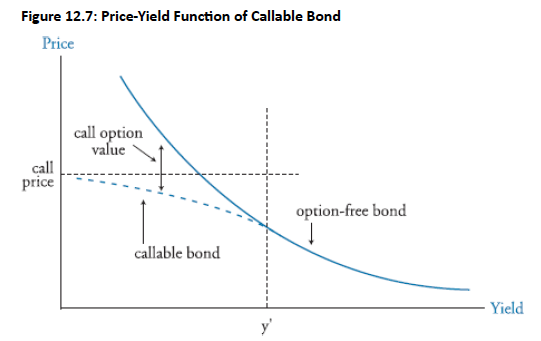
- Definition: A callable bond includes a call feature allows the issuer to repurchase the bond at fixed prices before maturity, giving the issuer (not the investor) the right to buy back the bond.
- Callable bonds exhibit negative convexity when yields fall below a certain level (y′), causing the price-yield curve to flatten rather than rise indefinitely as it would for noncallable bonds.
- Negative convexity occurs because the call price effectively caps the bond's market value, limiting investors' capital gains as yields decline.
- At yield levels above y′, callable bonds behave like noncallable bonds and display positive convexity since the likelihood of being called is minimal. Below yield level y′, investors anticipate potential calls, which causes price compression as the bond's value is bounded by the call price rather than rising with falling yields.
- Callability increases reinvestment risk by forcing investors to reinvest both coupon payments and the call price at lower prevailing rates when the bond is called.
-
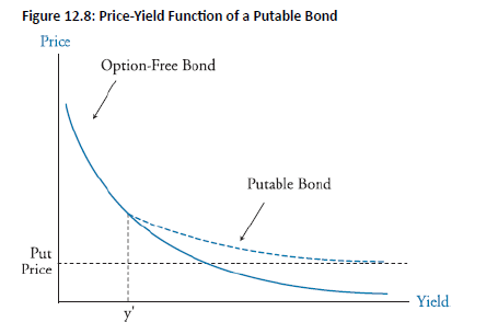
Definition: A putable bond includes a put feature that gives the bondholder the right to sell the bond back to the issuer at a predetermined price, with the investor holding the option to exercise.
- At low yield levels (below y′), putable bonds behave similarly to nonputable bonds in their price-yield relationship.
- When yields rise above y′, putable bonds decline in price more slowly than option-free bonds because the put price establishes a floor value for the bond's price.
- The put feature protects investors from significant price declines in rising rate environments by allowing them to sell the bond back at the put price.
Topic 5. Putable Bonds
Practice Questions: Q3
Q3. Which of the following statements about callable bonds compared to noncallable bonds is false?
A. They have less price volatility.
B. They have negative convexity.
C. Capital gains are capped as yields rise.
D. At low yields, reinvestment rate risk rises.
Practice Questions: Q3 Answer
Explanation: C is correct.
Callable bonds have the following characteristics:
- Less price volatility
- Negative convexity
- Capital gains are capped as yields fall
- Exhibit increased reinvestment rate risk when yields fall
Copy of MR 12. Arbitrage Pricing with Term Structure Models
By Prateek Yadav


