Book 1. Market Risk
FRM Part 2
MR 14. Art of Term Structure Models- Drift
Presented by: Sudhanshu
Module 1. Term Structure Models
Module 2. Arbitrage-Free Models
Module 1. Term Structure Models
Topic 1. Overview of Term Structure Models
Topic 2. Model 1 (No Drift): Overview
Topic 3. Model 1 (No Drift): Example
Topic 4. Model 1 (No Drift): Tree Construction
Topic 5. Model 1 (No Drift): Negative Rates
Topic 6. Model 1 (No Drift): Model Appropriateness
Topic 7. Model 1 (No Drift): Effectiveness
Topic 8. Model 2 (Constant Drift): Overview
Topic 9. Model 2 (Constant Drift): Effectiveness
Topic 10. Ho-Lee Model (Time-Dependent Drift)

Topic 1. Overview of Term Structure Models
- Purpose: Model short-term interest rate dynamics to price bonds, options, and derivatives.
-
Models differ in drift assumptions:
- Model 1: No Drift
- Constant Drift
- Time-Dependent Drift (Ho-Lee)
- Mean-Reverting Drift (Vasicek)
Topic 2. Model 1 (No Drift): Overview
-
General Form:
- : change in interest rates over small time interval dt
- : small time interval (measured in years) (e.g. one month =1/12)
- : annual basis point volatility of rate changes,
- : normally distributed random variable with mean 0 and standard deviation
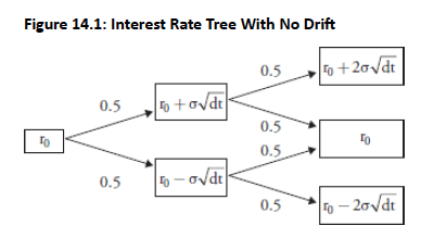
- Binomial Tree: Built using equal 50% probability for up and down movements in each period
- Recombining Property: Tree structure where up-down path equals down-up path, both ending at same node in second period
- Same movement probabilities maintained across all time periods in the model
- No Drift: Since the expected value of dw is zero [i.e., E(dw) = 0], the drift will be zero.
- Standard Deviation of the rate: Since the standard deviation of dw = , the volatility of the rate change =. . This is also known as standard deviation of the rate.
d w
dr
\sigma
dr=\sigma dw
dt
\sqrt{dt}
\sqrt{dt}
\sigma\sqrt{dt}
- Consider the evolution of interest rates on a monthly basis.
-
Let
-
Therefore, dw has a mean of 0 and standard deviation of
-
- After 1 month, let dw = 0.2 (drawn from a normal distribution with mean 0 and standard deviation of 0.2887). Therefore, dr = 1.20% × 0.2 = 0.24% = 24 basis points.
- Since was & it changed by 0.24%, the new spot rate in 1 month= 6% + 0.24% = 6.24%.
- The standard deviation of the rate=
-
The terminal nodes in the two-period model generate three possible ending rates:
-
-
This discrete finite outcomes don't technically represent normal distribution, but terminal node distribution approaches continuous normal distribution as number of steps increases
-
Topic 3. Model 1 (No Drift): Example
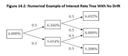
r_0=6 \%, \sigma = 1.20\%, dt=1/12
\sqrt{1/dt}=0.2887.
\sigma\sqrt{dt} = 1.2 \% \times \sqrt{1 / 12}=0.346 \%=34.6 \text{ basis points}
r_0=6 \%
r_0+2\sigma \sqrt{dt}, r_0, \text{ and } r_0-2\sigma \sqrt{dt}
- We will consider a two-period recombining tree: This tree is recombining and the ending rate at time 2 for the middle node is the same as the initial rate, implying no drift.
-
1 period from now, the interest rate will either increase (or decrease) with 50% probability to: 6% + 0.346% = 6.346% ( or 6% − 0.346% = 5.654%)
-
Extending to two periods completes the tree with upper node: 6% +2(0.346%) = 6.692%, middle node: 6% (unchanged), and lower node: 6% − 2(0.346%) = 5.308%
-
The terminal nodes in the two-period model generate three possible ending rates:
-
-
This discrete finite outcomes don't technically represent normal distribution, but terminal node distribution approaches continuous normal distribution as number of steps increases
-
Topic 4. Model 1 (No Drift): Tree Construction
r_0+2\sigma \sqrt{dt}, r_0, \text{ and } r_0-2\sigma \sqrt{dt}
- Negative Rate Risk: Model 1 always has positive probability that interest rates could become negative, which lacks obvious economic rationale
- Economic Irrationality: Negative rates imply lending $100 and receiving less than $100 back, contradicting normal lending economics
- Possible Justification: Small negative rates could be rationalized if cash holding involves sufficiently high safety costs or inconvenience factors
- Time Horizon Effect: Negative interest rate problem worsens with longer investment horizons as probability of forecasted rates dropping below zero increases
-
Solutions to negative rates:
- Non-Negative Distributions: Use always positive distributions like lognormal or chi-squared to prevent negative rates, though this may introduce undesirable skewness or inappropriate volatilities
- Zero Floor Method: Force negative rates to zero value, adjusting the original tree to constrain distribution below zero
- Preferred Approach: Zero floor method typically preferred as it only modifies distribution in very low rate environments, while changing entire distribution affects much wider range of rates
Topic 5. Model 1 (No Drift): Negative Rates
-
Users must ultimately decide if the model suits their specific purpose and risk tolerance for negative rates
- Bond Pricing Applications: Coupon-paying bond valuations depend on average rates over bond life, making small probability of negative rates less critical
- Option Valuation Concerns: Models with asymmetric payoffs are more significantly affected by negative interest rate problems than linear instruments
Topic 6. Model 1 (No Drift): Model Appropriateness
- Given the no-drift assumption of Model 1, we can draw several conclusions regarding the effectiveness of this model
- Limited Term Structure Flexibility: No-drift assumption creates insufficient flexibility for accurate modeling, resulting in downward-sloping predicted term structure due to larger convexity effects
- Flat vs. Hump-Shaped Volatility: Model 1 predicts flat volatility term structure while observed volatility is hump-shaped (rising then falling)
- Single Factor Limitation: Model uses only short-term rate factor, while richer models incorporate additional factors like drift and time-dependent volatility
- Parallel Shift Problem: Model implies short-rate changes cause parallel yield curve shifts, contradicting observed nonparallel yield curve movements
Topic 7. Model 1 (No Drift): Effectiveness
Topic 8. Model 2 (Constant Drift): Overview
- Casual observation of term structures typically reveals upward-sloping yield curves
- In Model 2, a constant drift is added to Model 1 that can be interpreted as a positive risk premium associated with long time horizons
-
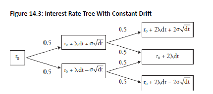
Model 2 Equation:
- Introduces deterministic upward trend via drift λ\lambdaλ.
- Tree is still recombining but centers shift upward over time.
-
Example: λdt+σdwdr = \lambda dt + \sigma dw
-
The monthly drift = 0.24%×1/12 = 0.02% & the sd of the rate
- The monthly drift represents expected change + risk premium.
- The drift term term increases by λdt in each period, making the yield curve upward-sloping
- Note: The tree recombines at time 2, but the rate at middle node is greater than original rate
d r=\lambda d t+\sigma d w
r_0=5 \%, \lambda=0.24 \%, \sigma=1.5 \%, d t=1 / 12, d w=0.2
\text { Drift }=0.02 \%, \text { Volatility }=0.3 \% \Rightarrow d r=0.32 \%, r_1=5.32 \%
=1.5 \% \times \sqrt{1 / 12}=0.43 \%
Topic 9. Model 2 (Constant Drift): Effectiveness
- Superior Performance: Model 2 outperforms Model 1 by incorporating drift term that accommodates typically observed upward-sloping yield curves
- Calibration Benefits: Researchers can choose r₀ and λ parameters based on observed rate calibration, resulting in better term structure fit
- High Drift Concern: Estimated drift values could be relatively high if interpreted solely as risk premium component
- Combined Interpretation: Viewing drift as combination of risk premium and expected rate changes suggests rates increase over time (e.g., Year 10 higher than Year 9), which is more appropriate for short-term analysis
Topic 10. Ho-Lee Model (Time-Dependent Drift)
- Allows drift to vary by time period ⇒ more realistic modeling.
- Equation:
-
Tree Properties:
- Recombining.
- Drift values are calibrated to match observed market yields.
- Can handle downward or flat yield curves too.
- Greater calibration accuracy for multi-period pricing.
- More general than Model 2 (Model 2 is a special case if
d r=\lambda(t) d t+\sigma d w
\left(\lambda_1, \lambda_2, \ldots\right)
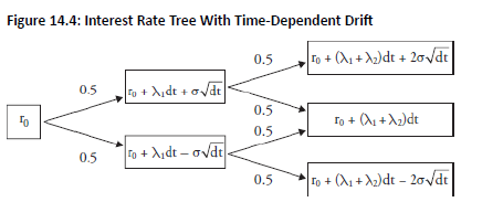
\left.\lambda_1=\lambda_2=\ldots\right)
Practice Questions: Q1
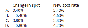
Q1. Using Model 1, assume the current short-term interest rate is 5%, annual volatility is 80bps, and dw, a normally distributed random variable with mean 0 and standard deviation, , has an expected value of zero. After one month, the realization of dw is −0.5. What is the change in the spot rate and the new spot rate?
\sqrt{d t}
Practice Questions: Q1 Answer
Explanation: B is correct.
Model 1 has a no-drift assumption. Using this model, the change in the interest rate is predicted as:
basis points
Since the initial rate was 5% and dr = −0.40%, the new spot rate in one month is: 5% − 0.40% = 4.60%
\begin{aligned}
& \mathrm{dr}=\sigma \mathrm{dw} \\
& \mathrm{dr}=0.8 \% \times(-0.5)=-0.4 \%=-40
\end{aligned}
Practice Questions: Q2
Q2. Using Model 2, assume a current short-term rate of 8%, an annual drift of 50bps, and a short-term rate standard deviation of 2%. In addition, assume the ex-post realization of the dw random variable is 0.3. After constructing a 2-period interest rate tree with annual periods, what is the interest rate in the middle node at the end of Year 2?
A. 8.0%.
B. 8.8%.
C. 9.0%.
D. 9.6%.
Practice Questions: Q2 Answer
Explanation: C is correct.
Using Model 2 notation:
- current short-term rate,
- drift,
- standard deviation,
- random variable,
- change in time,
Since we are asked to find the interest rate at the second period middle node using Model 2, we know that the tree will recombine to the following rate:
r_0=8 \%
\lambda=0.5 \%
\sigma=2 \%
d w=0.3
\mathrm{dt}=1
\mathrm{r}_0+ 2 \lambda \mathrm{dt} = 8\% + 2 × 0.5\% × 1 = 9\%
Module 2. Arbitrage-Free Models
Topic 1. Arbitrage-Free Models: Overview
Topic 2. Vasicek Model: Mean Reversion
Topic 3. Vasicek Model: Non-Recombining Tree
Topic 4. Vasicek Model: Recombining Tree
Topic 5. Vasicek Model: Rate Change, SD of Rate Change and Half-Life
Topic 6. Vasicek Model Effectiveness
Topic 1. Arbitrage-Free Models: Overview
-
Two main model types: Arbitrage-free models and equilibrium models.
-
Key distinction: Choice depends on the need to match market prices.
-
Arbitrage-free models:
-
Calibrated to match observable market prices (e.g., on-the-run Treasuries).
-
Used to price illiquid/custom securities and derivatives (e.g., bond options).
-
Limitations:
-
Calibration depends on suitability of the pricing model (e.g., parallel shift assumption).
-
Relies on accurate market prices; can be distorted by temporary external shocks.
-
-
-
Equilibrium models:
-
Preferred for relative analysis when comparing securities;
-
Arbitrage-free models are meaningless if prices are temporarily distorted.
-
Topic 2. Vasicek Model: Mean Reversion
- The Vasicek model assumes a mean-reverting process for short-term interest rates.
- The economy has a long-run equilibrium rate driven by fundamentals (e.g., monetary supply, technology).
-
Drift adjustment logic:
-
If rates are above equilibrium → negative drift to pull them down.
-
If rates are below equilibrium → positive drift to push them up.
-
-
Mean reversion assumption works in normal conditions but fails during structural breaks like hyperinflation.
-
Equation:
- : Long-run equilibrium rate
- k: Speed of mean reversion
-
Interpretation:
-
k measures mean reversion speed; higher k → faster/larger adjustments.
-
Larger gap between long-run and current rates → bigger adjustment.
-
Drift term (λ) combines expected rate change and risk premium.
-
Under risk neutrality, long-run short rate θ can be approximated accordingly.
-
d r=k(\theta-r) d t+\sigma d w
\theta
Topic 3. Vasicek Model: Non-Recombining Tree
-
Example:
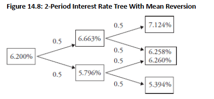
- Monthly drift: 0.03(18−6.2)/12=0.0295%0.03(18 - 6.2)/12 = 0.0295\%0.03(18−6.2)/12=0.0295%
- Monthly volatility:
- Show asymmetry: up-down ≠ down-up ⇒ non-recombining tree
- Due to variable size of drift based on how far node is from
-
Starting with , the interest rate tree over the first period is:
r_0=6.2 \%, k=0.03, \sigma=1.5 \%,\theta= 6\%+\frac{0.36 \%}{3}= 18 \%,
1.5 \% / \sqrt{12}=0.43 \%
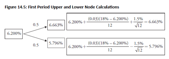
r_0=6.2\%
Topic 3. Vasicek Model: Non-Recombining Tree
-
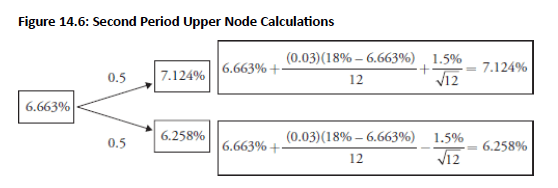
If rates rise in the first period, move to the upper node in period two.
-
In the second period, rate can go up to 7.124% or down to 6.258%.
-
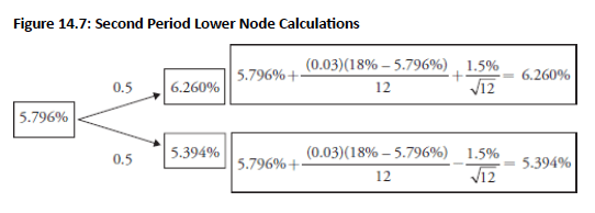
If rates falls in the first period, move to the lower node in period two.
-
In the second period, rate can go up to 6.260% or down to 5.394%.
Topic 3. Vasicek Model: Non-Recombining Tree
- The 2-period interest rate tree with mean reversion is non-recombining.
- Up-down path: 6.258% rate; down-up path: 6.260% rate.
- Down-up path rate > up-down path rate due to larger mean reversion adjustment from the lower initial rate (5.796% vs. 6.663%).
Topic 4. Vasicek Model: Recombining Tree
-
Vasicek model initially produces a 2-period non-recombining tree of short-term rates.
-
A recombining tree can be created using a modified method.
-
Step 1: Average the two middle nodes: (6.258% + 6.260%) / 2 = 6.259%.
-
Step 2: Replace 50/50 up-down probabilities with (p, 1−p) and (q, 1−q).
-
Solve for p and q (probabilities of up moves in period 2 after an up or down move in period 1).
-
-
Interest rates from successive moves (up-up and down-down) in the tree
-
Solve unknowns (p, q, ) using a system of equations.
-
Equation 1: p×ruu+(1−p)×6.259%=6.691%p \times ruu + (1-p) \times 6.259\% = 6.691\%
-
Equation 2: Use the standard deviation definition to form the second equation.
-
-
Repeat the process for the bottom portion of the tree, solving for q and
-
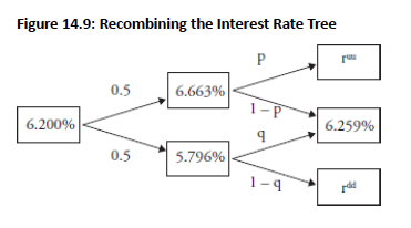
r^{uu} \text{ and } r^{dd}:
r^{uu}, r^{dd}
p \times r^{u u}+(1-p) \times 6.259 \%=6.691 \%
\sqrt{\mathrm{p}\left(\mathrm{r}^{\mathrm{uu}}-6.691 \%\right)^2+(1-\mathrm{p})(6.259 \%-6.691 \%)^2}=1.50 \% \times \sqrt{\frac{1}{12}}
r^{dd}
Topic 5. Vasicek Model: Rate Change, SD of Rate Change and Half-Life
-
Expected Rate in TTT years: Weighted average of current short-term rate and its long-run horizon value.
-
-
Factor's half-Life: Number of years to close half the distance between the starting rate and mean-reverting level.
-
A larger mean reversion adjustment parameter, k, will result in a shorter half-life.
r_T=r_0 e^{-k T}+\theta\left(1-e^{-k T}\right)
\tau=\frac{\ln 2}{k}
Topic 6. Vasicek Model Effectiveness
- Calibration and Volatility Structure: Mean-reverting (Vasicek) model calibrates r₀ and θ to market prices, producing declining volatility term structure that overstates short-term and understates long-term volatility
- Flat Volatility Comparison: Model 1 (no drift) generates flat volatility across all maturities, contrasting with Vasicek's declining pattern
- Non-Parallel Yield Shifts: Vasicek model shows short-term rates more impacted than long-term rates from upward shifts, avoiding parallel shift implications of non-mean-reverting models
- Shock Dissipation: Mean reversion causes short-term economic news shocks to dissipate toward long-run mean, with larger reversion parameters incorporating news faster
- Economic News Duration: Smaller mean reversion parameters indicate longer-lived economic news that takes more time to be assimilated into security prices
- Parallel Shift Problem: Models without drift cause shocks to affect all rates equally regardless of maturity, producing unrealistic parallel shifts
Practice Questions: Q1
Q1. The Bureau of Labor Statistics has just reported an unexpected short-term increase in high-priced luxury automobiles. What is the most likely anticipated impact on a mean-reverting model of interest rates?
A. The economic information is long-lived with a low mean reversion parameter.
B. The economic information is short-lived with a low mean reversion parameter.
C. The economic information is long-lived with a high mean reversion parameter.
D. The economic information is short-lived with a high mean reversion parameter.
Practice Questions: Q1 Answer
Explanation: D is correct.
The economic news is most likely short-term in nature. Therefore, the mean reversion parameter is high so the mean reversion adjustment per period will be relatively large.
Practice Questions: Q2
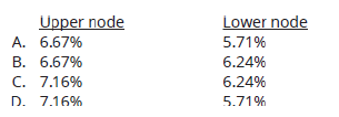
Q2. Using the Vasicek model, assume a current short-term rate of 6.2% and an annual volatility of the interest rate process of 2.5%. Also assume that the long-run mean-reverting level is 14.2% with a speed of adjustment of 0.4. Within a binomial interest rate tree, what are the upper and lower node rates after the first month?
Practice Questions: Q2 Answer
Explanation: D is correct.
Using a Vasicek model, the upper and lower nodes for Time 1 are computed as follows:
\begin{aligned}
& \text { upper node }=6.2 \%+\frac{(0.4)(13.2 \%-6.2 \%)}{12}+\frac{2.5 \%}{\sqrt{12}}=7.16 \% \\
& \text { lower node }=6.2 \%+\frac{(0.4)(13.2 \%-6.2 \%)}{12}-\frac{2.5 \%}{\sqrt{12}}=5.71 \%
\end{aligned}
Practice Questions: Q3
Q3. John Jones, FRM, is discussing the appropriate usage of mean-reverting models relative to no-drift models, models that incorporate drift, and Ho-Lee models. Jones makes the following statements:
-
Statement 1: Both Model 1 (no drift) and the Vasicek model assume parallel shifts from changes in the short-term rate.
-
Statement 2: The Vasicek model assumes decreasing volatility of future short-term rates while Model 1 assumes constant volatility of future short-term rates.
-
Statement 3: The constant drift model (Model 2) is a more flexible model than the Ho-Lee model.
How many of his statements are correct?
A. 0.
B. 1.
C. 2.
D. 3.
Practice Questions: Q3 Answer
Explanation: B is correct.
Only Statement 2 is correct. The Vasicek model implies decreasing volatility and nonparallel shifts from changes in short-term rates. The Ho-Lee model is actually more general than Model 2 (the no drift and constant drift models are special cases of the Ho-Lee model).
Copy of MR 14. Art of Term Structure Models- Drift
By Prateek Yadav


