


Sarah Dean PRO
asst prof in CS at Cornell
Fall 2025, Prof Sarah Dean
automated system
environment
action
measure-ment
training data \(\{(x_i, y_i)\}\)
model
\(p:\mathcal X\to\mathcal Y\)
features
predicted label
Notation
Training algorithms:
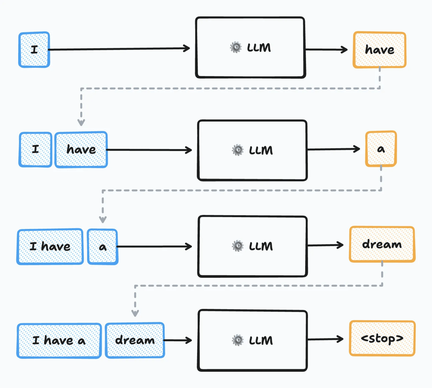
Auto-regressive models:
...
\(p_{\theta_2}:\mathcal X\to\mathcal Y\)
\(x_3\)
\(\hat y_3\) vs. \(y_3\)
\(p_{\theta_1}:\mathcal X\to\mathcal Y\)
\(x_2\)
\(\hat y_2\) vs. \(y_2\)
\(p_{\theta_0}:\mathcal X\to\mathcal Y\)
\(x_1\)
\(\hat y_1\) vs. \(y_1\)
training data
\(\{(x_i, y_i)\}\)
model
\(p:\mathcal X\to\mathcal Y\)
policy
observation
action
training data
\(\{(x_i, y_i)\}\)
model
\(p:\mathcal X\to\mathcal Y\)
observation
prediction
sampled i.i.d. from \(\mathcal D\)
\(x\sim\mathcal D_{x}\)
Goal: for new sample \(x,y\sim \mathcal D\), prediction \(\hat y = p(x)\) is close to true \(y\)
Notation
accumulate
\(\{x_t\}\)
model
\(p:\mathcal X^t\to\mathcal X\)
observation
prediction
\(x_t\sim\mathcal D_{t}\)
Goal: for new observation \(x\sim \mathcal D_t\), prediction \(\hat x_t\) is close to true \(x_t\)
Notation
model
\(p_t:\mathcal X\to\mathcal Y\)
observation
prediction
\(x_t\)
Goal: cumulatively over time, predictions \(\hat y_t = p_t(x_t)\) are close to true \(y_t\)
accumulate
\(\{(x_t, y_t)\}\)
policy
\(\pi_t:\mathcal X\to\mathcal A\)
observation
action
\(x_t\)
Goal: cumulatively over time, actions \(\pi_t(x_t)\) achieve high reward
\(a_t\)
accumulate
\(\{(x_t, a_t, r_t)\}\)
Notation
policy
\(\pi_t:\mathcal X^t\to\mathcal A\)
observation
action
\(x_t\)
Goal: select actions \(a_t\) to bring environment to high-reward state
\(a_t\)
accumulate
\(\{(x_t, a_t, r_t)\}\)
Participation expectation: actively ask questions and contribute to discussions
What we do:
Initialize \(\theta_0\)
For \(t=0,...,T\)
Sample \(x_i, y_i\) from dataset $$\theta_{t+1} = \theta_t - \eta \nabla_\theta \ell(y_i, p_{\theta}(x_i))_{\theta=\theta_t}$$
Why we do it:
$$\widehat p \approx \arg\min_{p\in\mathcal P} \underbrace{\sum_{i=1}^N \ell(y_i, p(x_i))}_{\approx \mathbb E[\ell(y, p(x))]}, \quad\mathcal P = \{p_\theta | \theta\in\mathbb R^d\}$$
Recall the goal: for new sample \(x,y\sim \mathcal D\), prediction \(\hat y\) is close to true \(y\)
Ex - classification
\(\ell(y,\hat y)\) measures "loss" of predicting \(\hat y\) when it's actually \(y\)
Ex - regression
Claim: The predictor with the lowest possible risk is
The risk of a predictor \(p\) over a distribution \(\mathcal D\) is the expected (average) loss
$$\mathcal R(p) = \mathbb E_{x,y\sim\mathcal D}[\ell(y, p(x))]$$
Proof: exercise. Hint: use tower property of expectation.
Goal: for new sample \(x,y\sim \mathcal D\), prediction \(\hat y = p(x)\) is close to true \(y\)
\(\ell(y,\hat y)\) measures "loss" of predicting \(\hat y\) when it's actually \(y\)
\(\implies\) Encode our goal in risk minimization framework:
$$\min_{p\in\mathcal P}\mathcal R(p) = \mathbb E_{x,y\sim\mathcal D}[\ell(y, p(x))]$$
\(\approx \mathcal R_N(p) = \frac{1}{N}\sum_{i=1}^N \ell(x_i,y_i)\)
1. Representation
2. Optimization
3. Generalization
\(\implies\) Solve with iterative algorithms (e.g. gradient descent) on the empirical risk
Next time: deep dive with least-squares
By Sarah Dean


