


Sarah Dean PRO
asst prof in CS at Cornell
Prof Sarah Dean
training data
\(\{(x_i, y_i)\}\)
model
\(f:\mathcal X\to\mathcal Y\)
policy
observation
action
model
\(f_t:\mathcal X\to\mathcal Y\)
observation
prediction
\(x_t\)
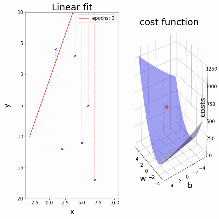
Goal: cumulatively over time, predictions \(\hat y_t = f_t(x_t)\) are close to true \(y_t\)
accumulate
\(\{(x_t, y_t)\}\)
$$\theta_t = \underbrace{\Big(\sum_{k=1}^{t-1}x_k x_k^\top + \lambda I\Big)^{-1}}_{A_{t-1}^{-1}}\underbrace{\sum_{k=1}^{t-1}x_ky_k }_{b_{t-1}}$$
Follow the (Regularized) Leader
$$\theta_t = \arg\min \sum_{k=1}^{t-1} (\theta^\top x_k-y_k)^2 + \lambda\|\theta\|_2^2$$
Online Gradient Descent
$$\theta_t = \theta_{t-1} - \alpha (\theta_{t-1}^\top x_{t-1}-y_{t-1})x_{t-1}$$
Sherman-Morrison formula: \(\displaystyle (A+uv^\top)^{-1} = A^{-1} - \frac{A^{-1}uv^\top A^{-1}}{1+v^\top A^{-1}u} \)
Follow the (Regularized) Leader
$$\theta_t = \arg\min \sum_{k=1}^{t-1} (\theta^\top x_k-y_k)^2 + \lambda\|\theta\|_2^2$$
Online Gradient Descent
$$\theta_t = \theta_{t-1} - \alpha (\theta_{t-1}^\top x_{t-1}-y_{t-1})x_{t-1}$$
Recursive FTRL
A world that evolves over time
$$ s_{t+1} = F(s_t)$$
(Autonomous) discrete-time dynamical system where \(F:\mathcal S\to\mathcal S\)
\(\mathcal S\) is the state space. The state is sufficient for predicting its future.
Given initial state \(s_0\), the solutions to difference equations, i.e. trajectories: $$ (s_0, F(s_0), F(F(s_0)), ... ) $$
What might trajectories look like?
An equilibrium point \(s_\mathrm{eq}\) satisfies
\(s_{eq} = F(s_{eq})\)
An equilibrium point \(s_{eq}\) is
examples:
Suppose that \(s_0=v\) is an eigenvector of \(A\)
$$ s_{t+1} = As_t$$
$$ s_{t} =\lambda^t v$$
Consider \(\mathcal S = \mathbb R^n\) and linear dynamics
Suppose that \(s_0=v\) is an eigenvector of \(A\)
$$ s_{t+1} = As_t$$
$$ s_{t} =\lambda^t v$$
Consider \(\mathcal S = \mathbb R^n\) and linear dynamics
\(\lambda>1\)
Consider \(\mathcal S = \mathbb R^n\) and linear dynamics
If similar to a real diagonal matrix: \(A=VDV^{-1} = \begin{bmatrix} |&&|\\v_1&\dots& v_n\\|&&|\end{bmatrix} \begin{bmatrix} \lambda_1&&\\&\ddots&\\&&\lambda_n\end{bmatrix} \begin{bmatrix} -&u_1^\top &-\\&\vdots&\\-&u_n^\top&-\end{bmatrix} \)
\(\displaystyle s_t = \sum_{i=1}^n v_i \lambda_i^t (u_i^\top s_0)\) is a weighted combination of (right) eigenvectors
$$ s_{t+1} = As_t$$
General case: real eigenvalues with geometric multiplicity equal to algebraic multiplicity
Example 1: \(\displaystyle s_{t+1} = \begin{bmatrix} \lambda_1 & \\ & \lambda_2 \end{bmatrix} s_t \)
\(0<\lambda_2<\lambda_1<1\)
\(0<\lambda_2<1<\lambda_1\)
\(1<\lambda_2<\lambda_1\)
Exercise: what do trajectories look like when \(\lambda_1\) and/or \(\lambda_2\) is negative? (demo notebook)
Example 2: \(\displaystyle s_{t+1} = \begin{bmatrix} \alpha & -\beta\\\beta & \alpha\end{bmatrix} s_t \)
\(0<\alpha^2+\beta^2<1\)
\(1<\alpha^2+\beta^2\)
Exercise: what do trajectories look like when \(\alpha\) is negative? (demo notebook)
General case: pair of complex eigenvalues
\(\lambda = \alpha \pm i \beta\)
$$\begin{bmatrix}1\\0\end{bmatrix} \to \begin{bmatrix}\alpha\\ \beta\end{bmatrix} $$
rotation by \(\arctan(\beta/\alpha)\)
scale by \(\sqrt{\alpha^2+\beta^2}\)
Example 3: \(\displaystyle s_{t+1} = \begin{bmatrix} \lambda & 1\\ & \lambda\end{bmatrix} s_t \)
\(0<\lambda<1\)
\(1<\lambda\)
Exercise: what do trajectories look like when \(\lambda\) is negative? (demo notebook)
General case: eigenvalues with geometric multiplicity \(>1\)
$$ \left(\begin{bmatrix} \lambda & \\ & \lambda\end{bmatrix} + \begin{bmatrix} & 1\\ & \end{bmatrix} \right)^t$$
$$ =\begin{bmatrix} \lambda^t & t\lambda^{t-1}\\ & \lambda^t\end{bmatrix} $$
All matrices are similar to a matrix of Jordan canonical form
where \(J_i = \begin{bmatrix}\lambda_i & 1 & &\\ & \ddots & \ddots &\\ &&\ddots &1\\ && &\lambda_i \end{bmatrix}\in\mathbb R^{m_i\times m_i}\)
Reference: Ch 3d and 4 in Callier & Desoer, "Linear Systems Theory"
\(\begin{bmatrix} J_1&&\\&\ddots&\\&&J_p\end{bmatrix} \)
\(m_i\) is geometric multiplicity of \(\lambda_i\)
Theorem: Let \(\{\lambda_i\}_{i=1}^n\subset \mathbb C\) be the eigenvalues of \(A\).
Then for \(s_{t+1}=As_t\), the equilibrium \(s_{eq}=0\) is
\(\mathbb C\)
Linearization via Taylor Series:
\(s_{t+1} = F(s_t) \)
Stability via linear approximation of nonlinear \(F\)
The Jacobian \(J\) of \(G:\mathbb R^{n}\to\mathbb R^{m}\) is defined as $$ J(x) = \begin{bmatrix}\frac{\partial G_1}{\partial x_1} & \dots & \frac{\partial G_1}{\partial x_n} \\ \vdots & \ddots & \vdots \\ \frac{\partial G_m}{\partial x_1} &\dots & \frac{\partial G_m}{\partial x_n}\end{bmatrix}$$
\(F(s_{eq}) + J(s_{eq}) (s_t - s_{eq}) \) + higher order terms
\(s_{eq} + J(s_{eq}) (s_t - s_{eq}) \) + higher order terms
\(s_{t+1}-s_{eq} \approx J(s_{eq})(s_t-s_{eq})\)
Consider the dynamics of gradient descent on a twice differentiable function \(g:\mathbb R^d\to\mathbb R^d\)
\(\theta_{t+1} = \theta_t - \alpha\nabla g(\theta_t)\)
Jacobian \(J(\theta) = I - \alpha \nabla^2 g(\theta)\)
if any \(\gamma_i\leq 0\), \(\theta_{eq}\) is not stable
i.e. saddle, local maximum, or degenerate critical point of \(g\)
Definition: A Lyapunov function \(V:\mathcal S\to \mathbb R\) for \(F,s_{eq}\) is continuous and
Reference: Bof, Carli, Schenato, "Lyapunov Theory for Discrete Time Systems"
Theorem (1.2, 1.4): Suppose that \(F\) is locally Lipschitz, \(s_{eq}\) is a fixed point, and \(V\) is a Lyapunov function for \(F,s_{eq}\). Then, \(s_{eq}\) is
Reference: Bof, Carli, Schenato, "Lyapunov Theory for Discrete Time Systems"
Theorem (3.3): Suppose \(F\) is locally Lipschitz, \(s_{eq}\) is a fixed point, and let \(\{\lambda_i\}_{i=1}^n\subset \mathbb C\) be the eigenvalues of the Jacobian \(J(s_{eq})\). Then \(s_{eq}\) is
Next time: actions, disturbances, measurement
References: Bof, Carli, Schenato, "Lyapunov Theory for Discrete Time Systems"; Callier & Desoer, "Linear Systems Theory"
By Sarah Dean


