Sarah Dean PRO
asst prof in CS at Cornell
(down arrow to see handout slides)
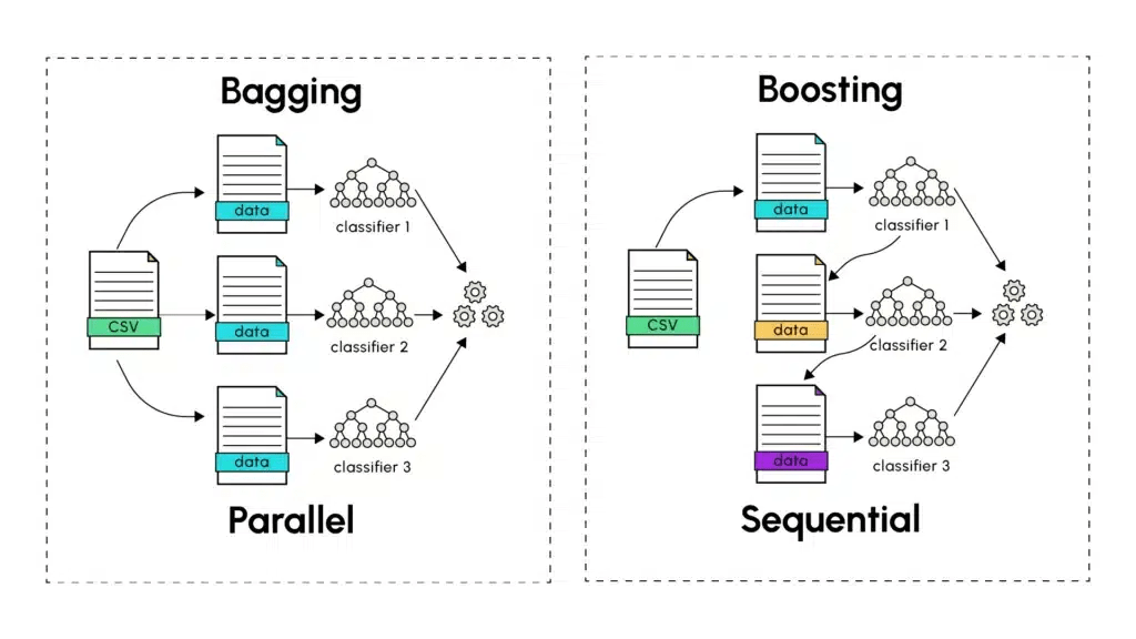
Ensemble Methods
Boosting Setting
Boosting Algorithm Idea
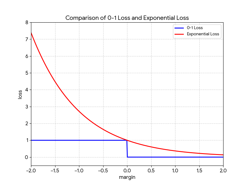
Adaboost Algorithm
Boosting Theorem
Proof Steps 1-4
Ensemble Methods
Boosting Setting
Boosting Algorithm Idea
Adaboost Algorithm
Boosting Theorem
Proof Steps 1-4
Ensemble Methods
Boosting Setting
Boosting Algorithm Idea
Adaboost Algorithm
Boosting Theorem
Proof Steps 1-4
Ensemble Methods
Boosting Setting
Boosting Algorithm Idea
Adaboost Algorithm
Boosting Theorem
Proof Steps 1-4
Since both \(h_t(\mathbf{x}_i),y_i \in \{-1, +1\}\), the product \(y_i h_t(\mathbf{x}_i)\) is always \(\pm 1\):
$$Z_t =\sum_{i:, h_t(\mathbf{x}i) = y_i} w_t[i] e^{-\alpha_t} + \sum_{i:, h_t(\mathbf{x}_i) \neq y_i} w_t[i] e^{\alpha_t}$$
Recall that $$\epsilon_t = \sum_{i=1}^{n} w_t[i] \mathbf{1}\{h_t(\mathbf x_i) \neq y_i\}, \quad \alpha_t = \frac{1}{2} \log\!\left(\frac{1 - \epsilon_t}{\epsilon_t}\right)$$
Ensemble Methods
Boosting Setting
Boosting Algorithm Idea
Adaboost Algorithm
Boosting Theorem
Proof Steps 1-4
By Sarah Dean


