

Sarah Dean PRO
asst prof in CS at Cornell
(down arrow to see handout slides)
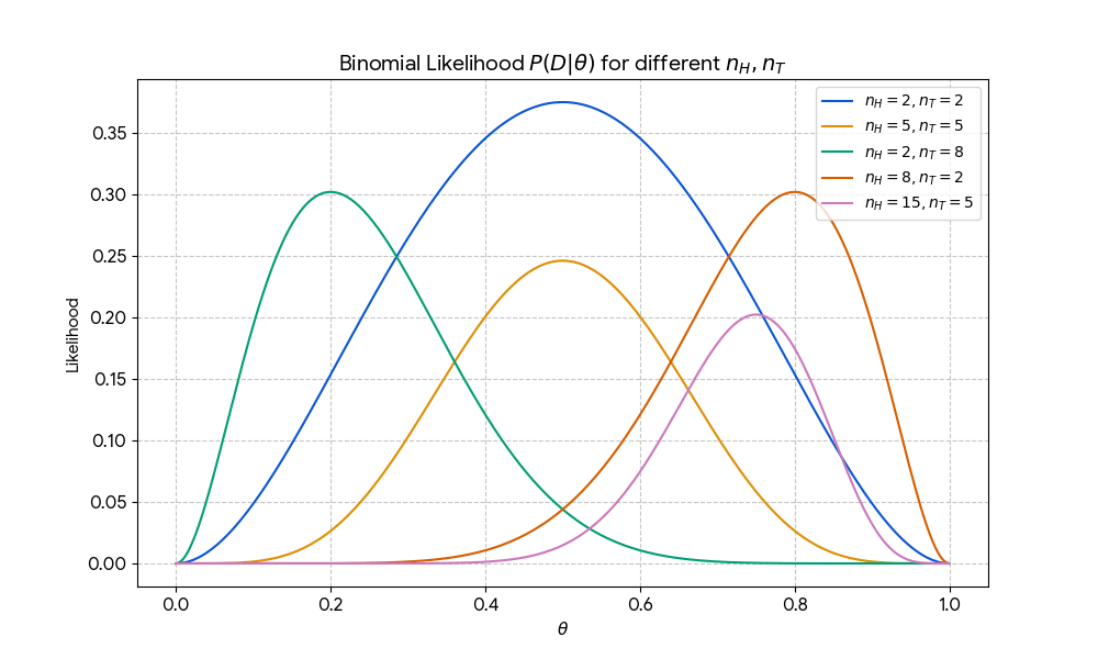
$$ P(D ; \theta) = \binom{n_H + n_T}{n_H} \theta^{n_H} (1-\theta)^{n_T} $$
Given training data \(D\), parameters \(\theta\), test point \(x_t\):
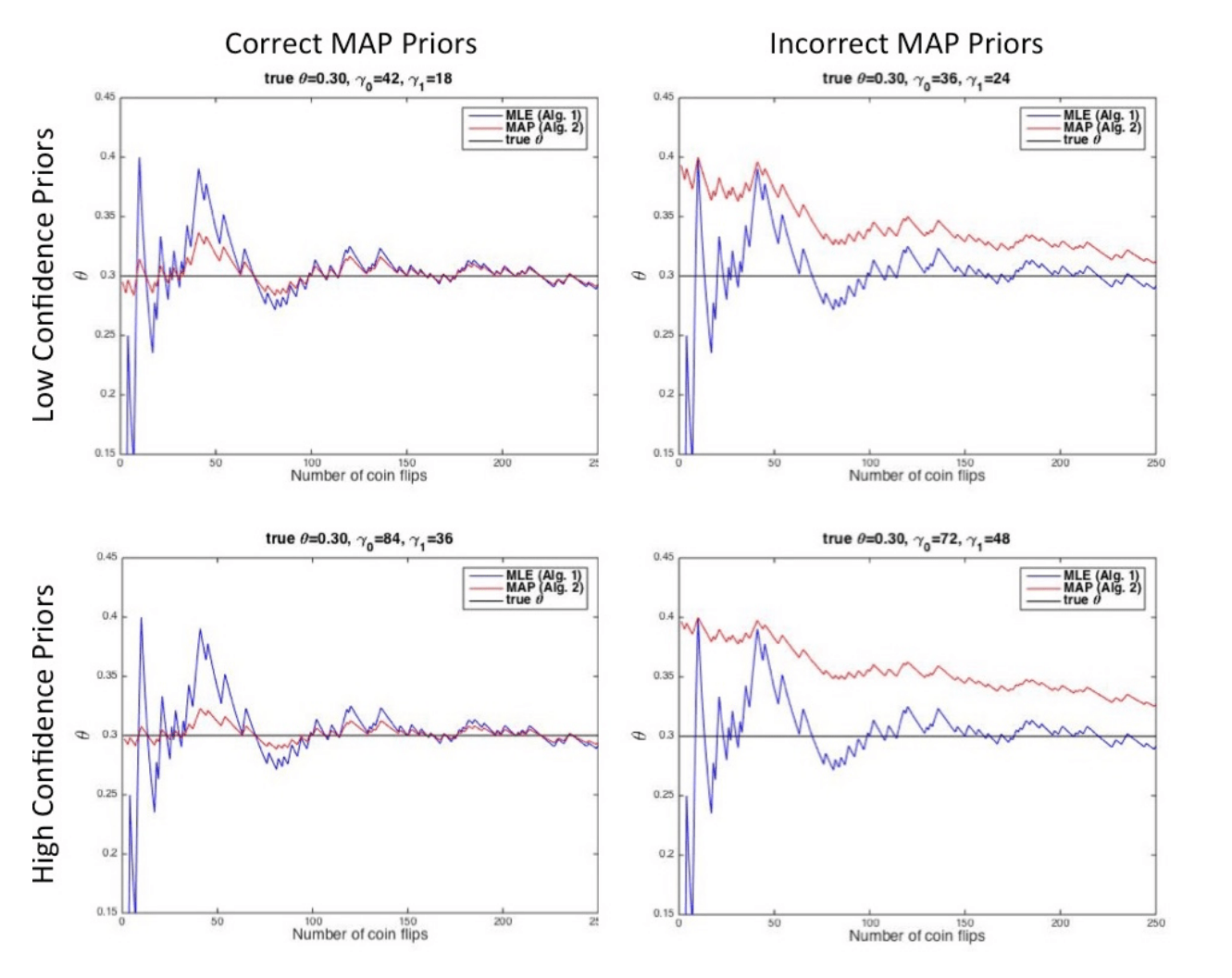
MLE:
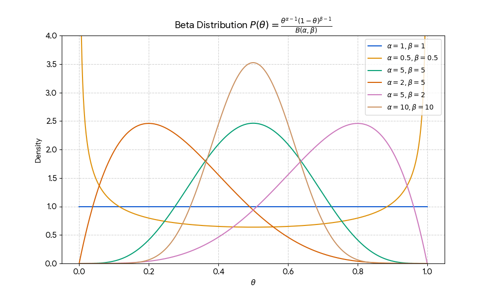
MAP:
Convergence: As \(n \to \infty\), \(\hat{\theta}_{MAP} \to \hat{\theta}_{MLE}\)
By Sarah Dean


