Learning and Control in the Presence of Observer Effects

Sarah Dean, Cornell University

IMSI Workshop, May 2026

Observer effects occur when there is coupling between actuation and observation

examples: electronic circuits, quantum wave collapse, human psychology, robotics ....

Observer Effects

Example: Personalization

$u_t$

unknown preference parameters $\theta$

expressed preferences

Example: Preference Dynamics

$u_t$

However, interests may be impacted by recommended content

preference state $x_t$

expressed preferences

Setting: Bilinearly Observed LDS

Setting: bilinearly observed linear dynamical system (BO-LDS)

Outline

1. Identification

2. Separation Principle

inputs

outputs

time

3. Optimal Control

Kalman

Filter

State Feedback

$y$

$\hat x$

$u$

Outline

i) Setting

ii) Algorithm

iii) Results

inputs

outputs

time

1. Identification from Bilinear Observations

Problem Setting: Identification

Unknown dynamics and measurement matrices $$A,B,C\quad\text{unkown}$$
Observed trajectory of inputs $u\in\mathbb R^p$ and outputs $y\in\mathbb R$ $$u_0,y_0,u_1,y_1,...,u_T,y_T$$
Goal: identify dynamics and measurement models from data

e.g. playlist attributes

e.g. listen time

inputs $u_t$

outputs $y_t$

Identification Algorithm

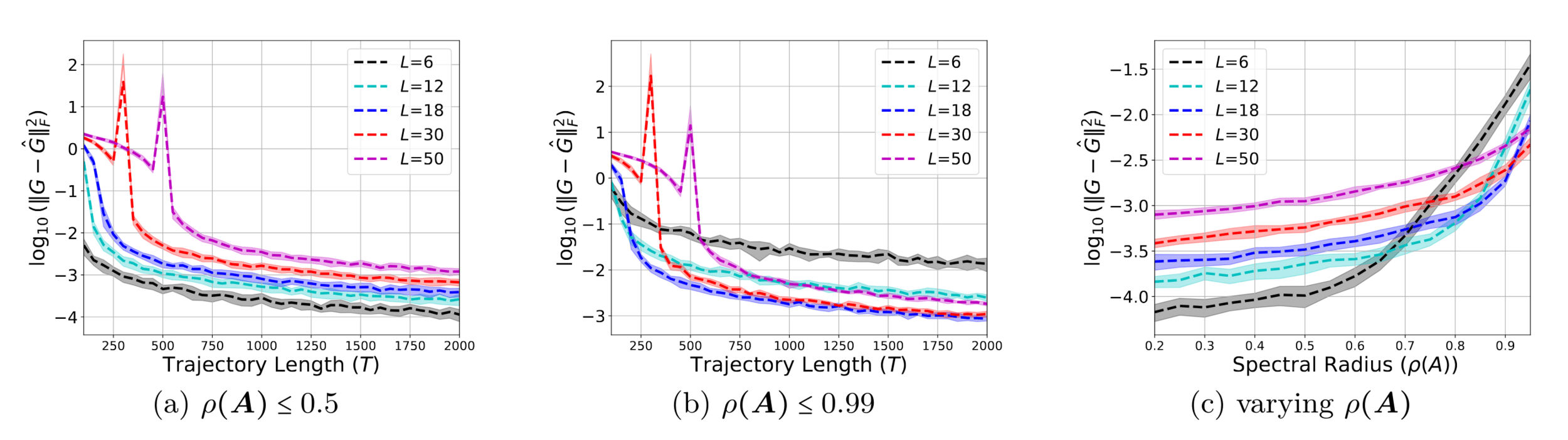
Input: data $(u_0,y_0,...,u_T,y_T)$, history length $L$, state dim $n$

Step 1: Regression

$$\hat G = \arg\min_{G\in\mathbb R^{p\times pL}} \sum_{t=L}^T \big( y_t - u_t^\top \textstyle \sum_{k=1}^L G[k] u_{t-k} \big)^2 $$

Step 2: Decomposition $\hat A,\hat B,\hat C = \mathrm{HoKalman}(\hat G, n)$
(Omyak & Ozay, 2019)

$t$

$L$

$\underbrace{\qquad\qquad}$

inputs

outputs

time

Yahya Sattar

$~$

Yassir Jedra

$$\underbrace{\qquad\qquad}_{} \\ \downarrow \\ \begin{bmatrix} u_{t-1}^\top & ... & u_{t-L}^\top \end{bmatrix} \otimes u_t^\top \mathrm{vec}(G) $$

degree 2 polynomial features

Estimation Errors

$$\hat G = \arg\min_{G\in\mathbb R^{p\times pL}} \sum_{t=L}^T \big( y_t - u_t^\top \textstyle \sum_{k=1}^L G[k] u_{t-k} \big)^2 $$

(Biased) estimate of Markov parameters $$ G =\begin{bmatrix} C B & CA B & \dots & CA^{L-1} B \end{bmatrix} $$
Regress $y_t$ against $$ \underbrace{ \begin{bmatrix} u_{t-1}^\top & ... & u_{t-L}^\top \end{bmatrix}}_{\bar u_{t-1}^\top } \otimes u_t^\top $$
Data matrix: circulant-like structure $$Z = \begin{bmatrix}\bar u_{L-1}^\top \otimes u_L^\top \\ \vdots \\ \bar u_{T-1}^\top \otimes u_T^\top\end{bmatrix} $$

$t$

$L$

$\underbrace{\qquad\qquad}$

$\bar u_{t-1}^\top \otimes u_t^\top \mathrm{vec}(G) $

inputs

outputs

time

Estimation Result

Under the following assumptions:

Process and measurement noise $w_t,v_t$ are i.i.d., zero mean, and have bounded second moments
Inputs $u_t$ are bounded
The dynamics are strictly stable, i.e. $\rho(A)<1$
(For state space recovery: $(A,B,C)$ are observable, controllable)

Informal Summary Theorem

Choosing $L=\log(T)/\log(\rho(A)^{-1})$ guarantees that with high probabilty, for bounded random design inputs $u_{0:T}$, $$\mathrm{estimation~errors} \lesssim \sqrt{ \frac{\mathsf{poly}(\mathrm{dimension})}{T}}$$

Main Results

Assumptions:

Process and measurement noise $w_t,v_t$ are i.i.d., zero mean, and have bounded second moments
Inputs $u_t$ are bounded
The dynamics are strictly stable, i.e. $\rho(A)<1$

Informal Theorem (Markov parameter estimation)

With probability at least $1-\delta$, $$\|G-\hat G\|_{Z^\top Z} \lesssim \sqrt{ \frac{p^2 L}{\delta} \cdot c_{\mathrm{stability,noise}} }+ \rho(A)^L\sqrt{T} c_{\mathrm{stability}}$$

$\hat G$

Proof Sketch

$$\hat G = \arg\min_{G\in\mathbb R^{p\times pL}} \sum_{t=L}^T \big( y_t - \bar u_{t-1}^\top \otimes u_t^\top \mathrm{vec}(G) \big)^2 $$

Claim: this is a biased estimate of Markov parameters $$ G_\star =\begin{bmatrix} C B & CA B & \dots & CA^{L-1} B \end{bmatrix} $$
- Observe that $x_t = \sum_{k=1}^L CA^{k-1} B (u_{t-k} + w_{t-k}) + A^L x_{t-L}$
- Hence, $y_t= \bar u_{t-1}^\top \otimes u_t^\top \mathrm{vec}(G_\star) +u_t^\top \textstyle \sum_{k=1}^L CA^{k-1} w_{t-k} + u_t CA^L x_{t-L} + v_t $
Least squares: for $y_t = z_t^\top \theta + n_t$, the estimate $\hat\theta=\arg \min\sum_t (z_t^\top \theta - y_t)^2$ $$= \textstyle\arg \min \|Z \theta - Y\|^2_2 = (Z^\top Z)^\dagger Z^\top Y= \theta_\star + (Z^\top Z)^\dagger Z^\top N$$
Estimation errors are therefore $\|G_\star -\hat G\|_{Z^\top Z} = \|Z^\top N\| $
Blocking technique to bound minimum singular value of $Z$

$*$

$=$

$$ = \begin{bmatrix}\bar u_{L-1}^\top \otimes u_L^\top \\ \vdots \\ \bar u_{T-1}^\top \otimes u_T^\top\end{bmatrix} =Z$$

Informal Summary Theorem

Analysis requires blocking technique for dependent covariates $$\begin{bmatrix} u_{t-1}^\top & ... & u_{t-L}^\top \end{bmatrix} \otimes u_t^\top$$
Open question: marginally stable $\rho(A)=1$?
- Regressing additionally against past outputs $y_{t-1:t-L}$ introduces higher order polynomial dependence (degree $L$)

Estimation Result

Outline

1. Identification

2. Separation Principle

inputs

outputs

time

3. Optimal Control

Kalman

Filter

State Feedback

$y$

$\hat x$

$u$

Outline

i) Control Setting

ii) SP Policy

2. Separation Principle for Control from Bilinear Obs

Kalman

Filter

State Feedback

$y$

$\hat x$

$u$

Problem Setting: Optimal Control

Linear state update with $A\in\mathbb R^{n\times n}$, $B\in\mathbb R^{n\times p}$ $$x_{t+1} = Ax_t + Bu_t + w_t $$
Bilinear measurements with $C_i\in\mathbb R^{m\times n}$ $$y_t = \underbrace{\Big(C_0 + \sum_{i=1}^p u_t[i] C_i \Big)}_{C(u_t)}x_t + v_t$$
Quadratic costs with $Q,R\succ 0$ $$c(x,u) = x^\top Q x + u^\top R u $$
Gaussian process noise, measurement noise, and initial state $$\{w_t\} \sim \mathcal N(0,\Sigma_w),\quad \{v_t\} \sim \mathcal N(0, \Sigma_v),\quad x_0 \sim \mathcal N(0,\Sigma_0)$$
Information set for decision-making $$\mathcal I_t = \{u_0,...,u_{t-1}, y_0, ..., y_{t-1}\}$$

Problem Setting: Optimal Control

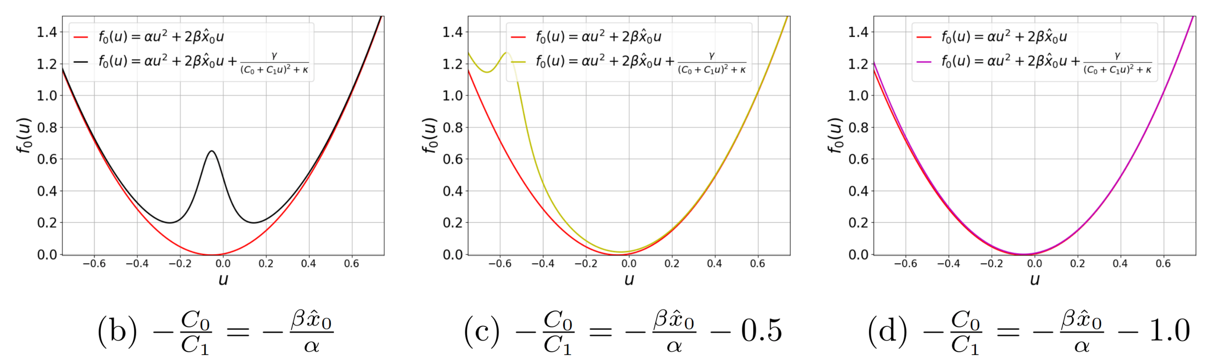
$$\min_{u_t=\pi_t(\mathcal I_t)} \mathbb E\left[x_T^\top Q x_T+ \sum_{t=1}^{T-1} x_t^\top Q x_t + u_t^\top R u_t \right]\\ \text{s.t.} \quad x_{t+1} = Ax_t + Bu_t + w_t \\\qquad\qquad\qquad y_t =\Big(C_0 + \sum_{i=1}^p u_t[i] C_i \Big)x_t + v_t$$

Small departure from classic LQG control

Sunmook Choi

Yahya Sattar

Yassir Jedra

Maryam Fazel

Leo Maynard-Zhang

Separation Principle

Separation principle (SP): independently design
estimation & control
- Optimal for partially observed
  LQ control ($C_i=0$ for $i>0$)
The SP policy has two components:
1. State estimation $\hat x_t = \mathbb E[x_t|\mathcal I_t]$
2. State dependent policy $u_t = K^\star_t \hat x_t$

Kalman

Filter

State Feedback

$y$

$\hat x$

$u$

Partial Observation LQ Control

Simplest problem: linear dynamics, quadratic cost, zero mean noise

$u_t = K_t^\star \hat x_t,\quad \hat x_t = \mathbb E[x_t|u_0,...,u_t,y_0,...,y_t]$

where $K^\star = \{K^\star_0,...,K^\star_T\}$ defined recursively depending on $A,B,Q,R$
and $\hat x_t$ depends on $A,B,C,\Sigma_w,\Sigma_v,\Sigma_0$
when noise is Gaussian, $\hat x_t$ computed efficiently with Kalman filter

Linear policy is optimal and can be computed in closed-form:

minimize $\mathbb{E}\left[ \sum_{t=0}^{T-1} x_t^\top Q x_t + u_t^\top R u_t\right]$

s.t. $x_{t+1} = Ax_t+Bu_t+w_t$

$y_{t} = Cx_t+v_t$

(separation principle)

Separation Principle Policy

The posterior distribution is given by the Kalman filter $x_t|\mathcal I_t \sim \mathcal N(\hat x_t,\Sigma_t)$

Open question: does $\varepsilon$ estimation error in dynamics lead to performance degradation scaling with $\varepsilon^2$ (as in LQG) or $\varepsilon$?

Conjecture: $\varepsilon$ (due to $\Sigma_t$), thus certainty equivalent control is not efficient

1. State Estimation with the Kalman Filter

$\hat x_{t+1} = A\hat x_t + Bu_t - L_t\big(y_t-C(u_t)\hat x_t\big)$

$\Sigma_{t+1} = (A+ L_tC(u_t))\Sigma_tA^\top + \Sigma_w$

$L_t = -A\Sigma_tC(u_t)^\top(C(u_t)\Sigma_tC(u_t)^\top+\Sigma_v)^{-1}$

2. State Feedback Control via LQR

$$u_t = K_t^\star \hat x_t$$

where $K^\star = \{K^\star_0,...,K^\star_T\}$ defined recursively depending on $A,B,Q,R$

Outline

1. Identification

2. Separation Principle

inputs

outputs

time

3. Optimal Control

Kalman

Filter

State Feedback

$y$

$\hat x$

$u$

Outline

i) SP is not Optimal

ii) Belief-space MPC

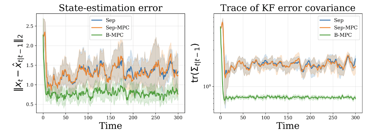
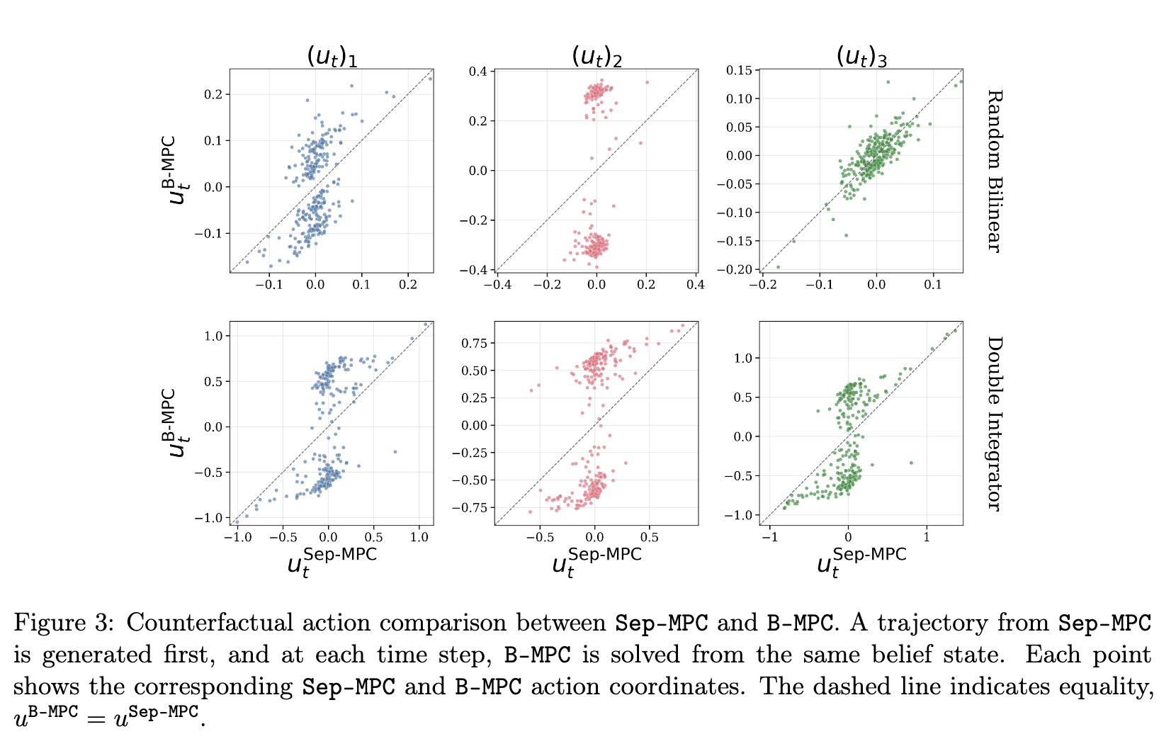
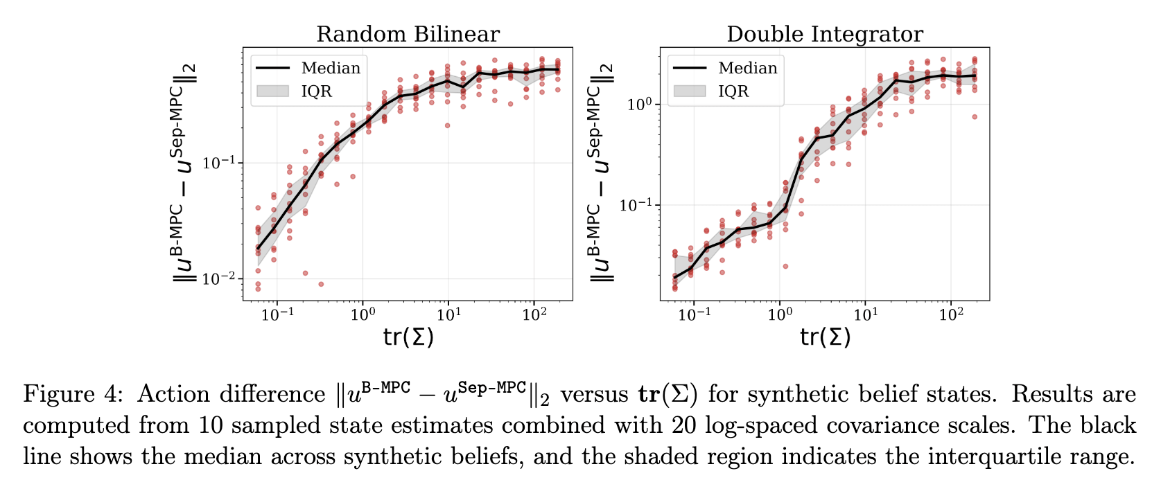
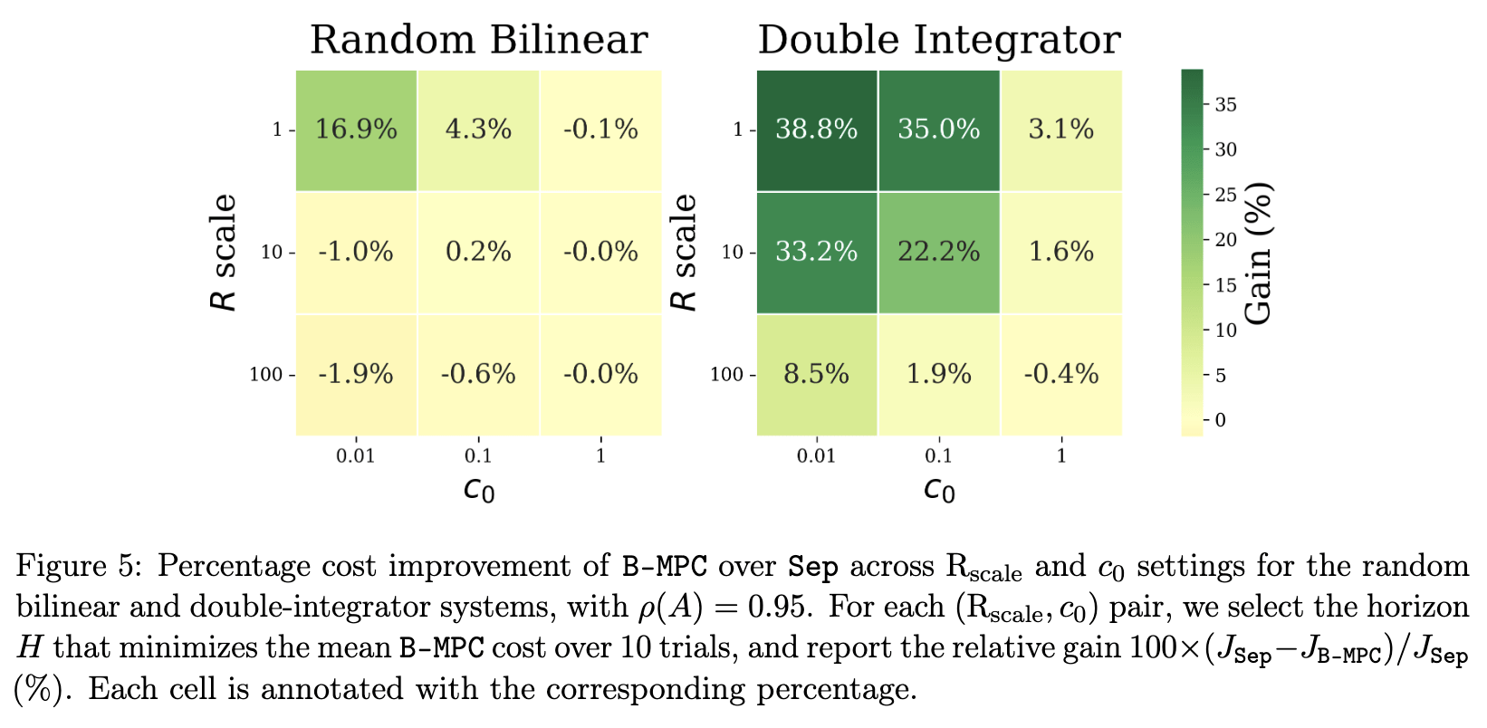
3. Optimal Control from Bilinear Observations

Optimality Results

Theorem: For $T\geq 2$, the optimal policy is not affine in the estimated state
- as a consequence, the SP policy is not optimal
Theorem: There exist instances in which the SP policy locally maximizes the cost
- in these instances, the optimal controller is nonlinear and not unique, i.e. for scalar system at $t=T-2$, $$ u^\star_{t} = -\alpha\hat x_{t}\left(1\pm \frac{1}{K_{t} \hat x_{t}}\sqrt{-\frac{\Sigma_z}{\Sigma_{t}} +\beta K_{t}}\right) $$

Proof Sketch

Strategy: analyze solution to dynamic programming
At $t=T$, the value function is $V_T(x) = x^\top Q x$
At $t=T-1$, $$V_{T-1}(x_t)= \min_u \underbrace{ \mathbb E[ c(x_t, u) +V_T(x_{t+1})|\mathcal I_{T-1}]}_{f_{T-1}(u) = f_{T-1}^\mathrm{LQ}(u)}$$
- The solution coincides with LQG $$u^\star_{T-1} = K^\star_{T-1}\mathbb E[x_{T-1}|\mathcal I_{T-1}]$$
At $t=T-2$, due to dependence of state estimation on input $$ \min_u\underbrace{\mathbb E[ c(x_t, u) +V_{T-1}x_{t+1})|\mathcal I_{T-2}]}_{f_{T-2}(u) = f_{T-2}^\mathrm{LQ}(u) + f^\mathrm{obs}_{T-2}(u)} $$

Proof Sketch

Strategy: analyze solution to dynamic programming
At $t=T$, the value function is $V_T(x) = x^\top Q x$
At $t=T-1$, $u^\star_{T-1} = K^\star_{T-1}\mathbb E[x_{T-1}|\mathcal I_{T-1}]$

At $t=T-2$, due to dependence of state estimation on input $$ \min_u\underbrace{\mathbb E[ c(x_t, u) +V_{T-1}x_{t+1})|\mathcal I_{T-2}]}_{f_{T-2}(u) = f_{T-2}^\mathrm{LQ}(u) + f^\mathrm{obs}_{T-2}(u)} $$

Examples where SP is bad

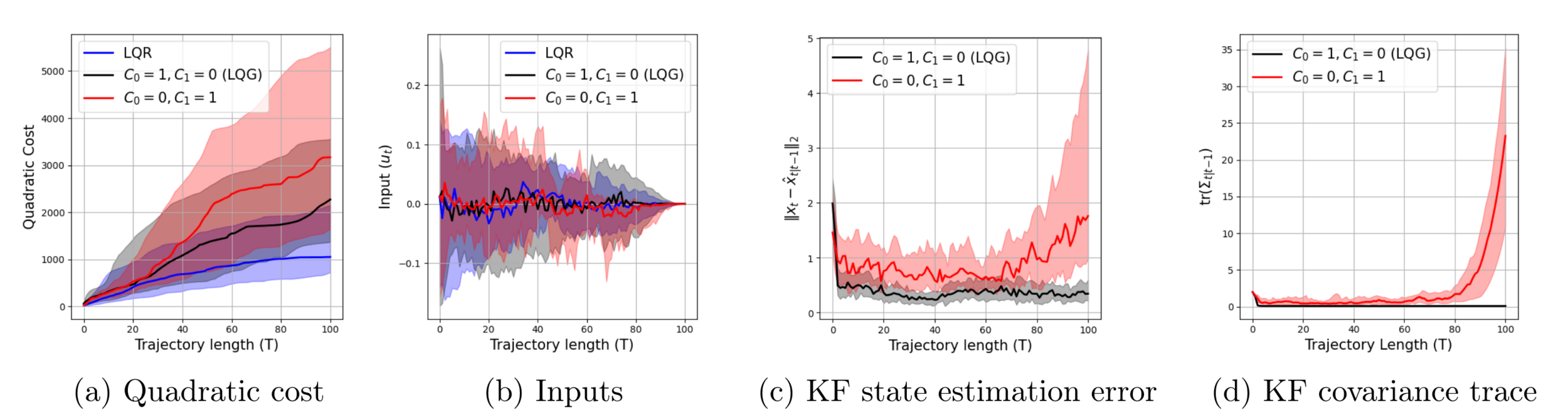
$$\begin{align*} x_{t+1} &= \begin{bmatrix} 1 & 0.3 \\ 0 & 1\end{bmatrix} x_t + \begin{bmatrix}0.3 \\ 0 \end{bmatrix} u_t + w_t \\ y_t &= u_t\begin{bmatrix} 1 & 0\end{bmatrix} x_t + v_t \end{align*}$$

with $Q=I$ and $R=1000$

$$\begin{align*} x_{t+1} &= x_t + \begin{bmatrix}0 & 1 \end{bmatrix} u_t + w_t \\ y_t &= u_t^\top \begin{bmatrix} 1\\ 0\end{bmatrix} x_t + v_t \end{align*}$$

with $Q=\frac{1}{2}$ and $R=I$

$\implies$

infinite horizon $K_\star = \begin{bmatrix} 0 \\ \frac{1}{2}\end{bmatrix}$

$y_t = \hat x_t \begin{bmatrix} 0 \\ \frac{1}{2}\end{bmatrix}^\top \begin{bmatrix} 1 \\ 0\end{bmatrix} x_t + v_t$

$0$ only noise is observed!

Belief Space Objective

Sunmook Choi

Yahya Sattar

$$\begin{align*}\min_{u_t=\pi_t(\hat x_t,\Sigma_t)}~~& \mathbb E\left[ \sum_{t=1}^{T-1} \hat x_t^\top Q \hat x_t + \mathrm{tr}(\Sigma_t) + u_t^\top R u_t \right]\\ \text{s.t.}~~& \hat x_{t+1} = A\hat x_t + Bu_t + L_t(C(u_t)\hat x_t - y_t)\\ &\Sigma_{t+1} = (A+ L_tC(u_t))\Sigma_tA^\top + \Sigma_w \end{align*}$$

$$\mathbb E\left[x_t^\top Q x_t \mid \mathcal I_t \right]= \hat x_t\top Q\hat x_t + \mathrm{tr}(Q\Sigma_t)$$

$$\begin{align*} \min_{u_t=\pi_t(\mathcal I_t)} ~~&\mathbb E\left[\sum_{t=1}^{T-1} x_t^\top Q x_t + u_t^\top R u_t \right]\\ \text{s.t.}~~& x_{t+1} = Ax_t + Bu_t + w_t \\& y_t =C(u_t)x_t + v_t\end{align*}$$

$L_t = -A\Sigma_tC(u_t)^\top(C(u_t)\Sigma_tC(u_t)^\top+\Sigma_v)^{-1}$

Andrew Lowitt

Beixi Du

Daniel Cao

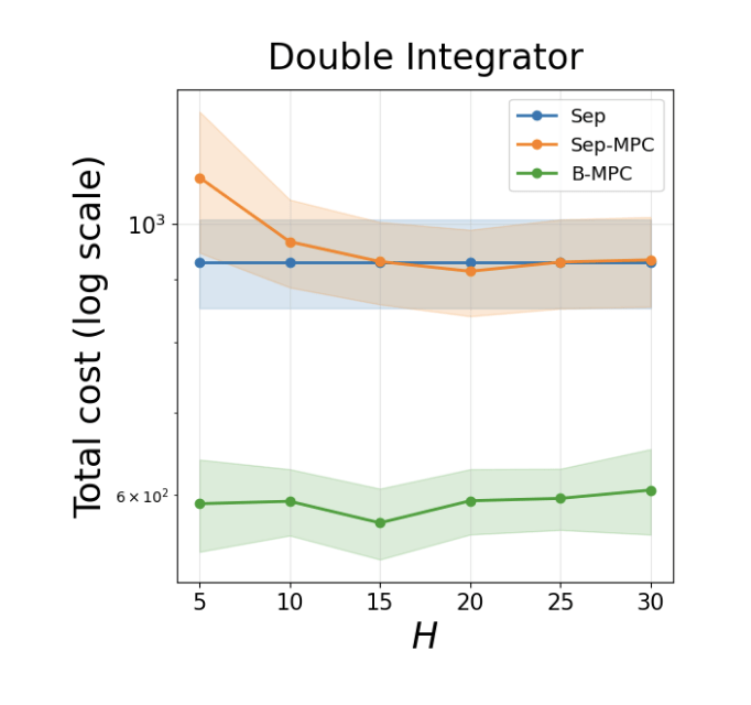
Rewrite OCP in terms of the belief space from KF

This is now a fully observed, nonlinear, stochastic optimal control problem

innovations $\sim \mathcal N(0, C(u_t)\Sigma_t C(u_t)^\top + \Sigma_v)$

Belief Space MPC

$$\begin{align*}\pi(\hat x_t,\Sigma_t)=\arg \min_{u_k}~~& \mathbb E\left[ \sum_{k=1}^{H} \bar x_k^\top Q \bar x_k + \mathrm{tr}(\bar\Sigma_k) + u_k^\top R u_k \right]\\ \text{s.t.}~~& \bar x_{k+1} = A\bar x_k + Bu_k\\ &\bar\Sigma_{k+1} = (A+ L_kC(u_k))\Sigma_kA^\top + \Sigma_w \\ &\bar x_0 = \hat x_t ,~~ \bar \Sigma_0=\Sigma_t\end{align*}$$

$L_t = -A\Sigma_tC(u_t)^\top(C(u_t)\Sigma_tC(u_t)^\top+\Sigma_v)^{-1}$

Rewrite OCP in terms of the belief space from KF

Expected dynamics, open loop inputs, finite horizon $\rightarrow$ MPC

"Solve" MPC problem with autograd and L-BFGS

Summary

1. Identification

2. Separation Principle

inputs

outputs

time

3. Optimal Control

Kalman

Filter

State Feedback

$y$

$\hat x$

$u$

$$x_{t+1} = Ax_t + Bu_t + w_t\qquad y_t = u_t^\top Cx_t + v_t$$

Stability is still crucial for identification

Bilinear observation changes the character of the learning and control problem

Certainty equivalent control may not be efficient

Optimal policy does not follow separation principle

What lessons did we learn about RL & ML-enabled control?

Simple model-based approaches work (no need for model-free)
Naive exploration is sufficient, or even no exploration
No need to account for finite sample uncertainty*

Lessons from LQ Control

$\implies$ Problem does not capture all issues of interest!

*Exceptions: low data regime, safety/actuation limits

Approach: ID then Control

1. Collect $N$ observations and estimate $\widehat A,\widehat B, \widehat C$

2. Design policy as if estimate is true ("certainty equivalent")

$(A_\star, B_\star,C_\star)$

$\widehat \pi$

$(A_\star, B_\star,C_\star)$

Control Result (Informal):

sub-opt. of $\widehat \pi\lesssim($param. err.$)^2 \lesssim \frac{1}{N}$

Learning Result (Informal):

parameter error $ \lesssim \frac{1}{\sqrt{N}}$

least squares regression

Naive exploration is essentially optimal!

white noise inputs

Learning Linear Dynamics from Bilinear Observations at ACC25 (arxiv:2409.16499) with Yahya Sattar and Yassir Jedra
Explore-then-Commit for Nonstationary Linear Bandits with Latent Dynamics at AISTATS26 (arxiv:2510.16208) with Sunmook Choi, Yahya Sattar, Yassir Jedra, Maryam Fazel
Sub-optimality of the Separation Principle for Quadratic Control from Bilinear Observations at CDC25 (arxiv:2504.11555) with Yahya Sattar, Sunmook Choi, Yassir Jedra, Maryam Fazel
Dual Control of Linear Systems from Bilinear Observations with Belief Space Model Predictive Control (arXiv:2604.24663) with Daniel Cao, Beixi Du, Andrew Lowitt, Sunmook Choi, Yahya Sattar

Thanks! Questions?

Sunmook Choi

Yahya Sattar

Yassir Jedra

Maryam Fazel

Leo Maynard-Zhang

Andrew Lowitt

Beixi Du

Daniel Cao

Learning and control in the presence of observer effects

By Sarah Dean

Learning and control in the presence of observer effects

Sarah Dean PRO

asst prof in CS at Cornell

sdean.website

Learning and Control in the Presence of Observer Effects

Sarah Dean, Cornell University

Observer Effects

Example: Personalization

Example: Preference Dynamics

Setting: Bilinearly Observed LDS

Outline

Outline

i) Setting

ii) Algorithm

iii) Results

Problem Setting: Identification

Identification Algorithm

Estimation Errors

Estimation Result

Informal Summary Theorem

Main Results

Informal Theorem (Markov parameter estimation)

Proof Sketch

Informal Summary Theorem

Estimation Result

Outline

Outline

i) Control Setting

ii) SP Policy

Problem Setting: Optimal Control

Problem Setting: Optimal Control

Separation Principle

Partial Observation LQ Control

Separation Principle Policy

Outline

Outline

i) SP is not Optimal

ii) Belief-space MPC

Optimality Results

Proof Sketch

Proof Sketch

Examples where SP is bad

Belief Space Objective

Belief Space MPC

Summary

Lessons from LQ Control

Approach: ID then Control

Thanks! Questions?

Learning and control in the presence of observer effects

More from Sarah Dean