
Sarah Dean PRO
asst prof in CS at Cornell
(down arrow to see handout slides)
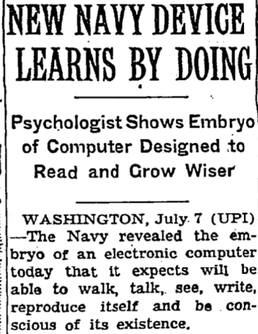
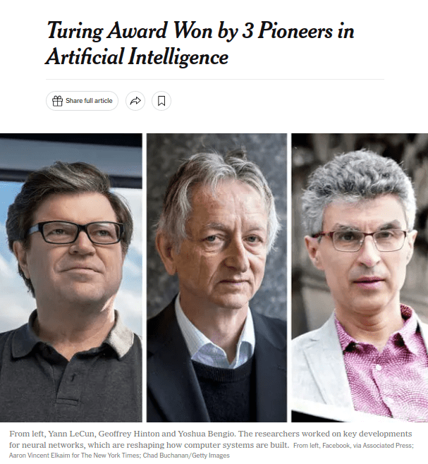
Frank Rosenblatt
New York Times, 1958
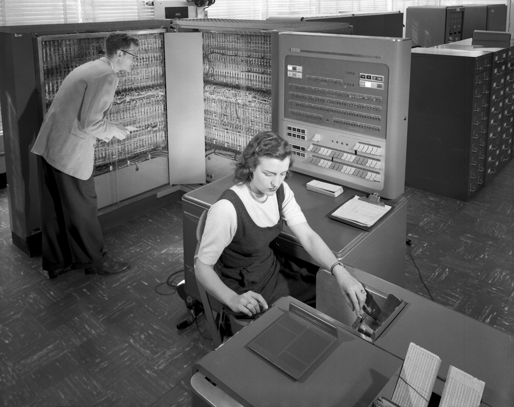
IBM 704
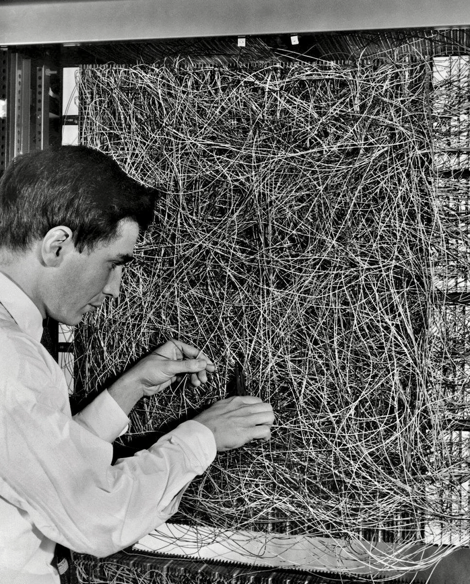
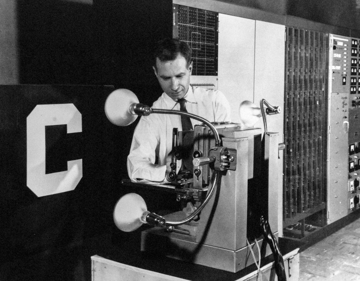
MARK I
Perceptron, 1960
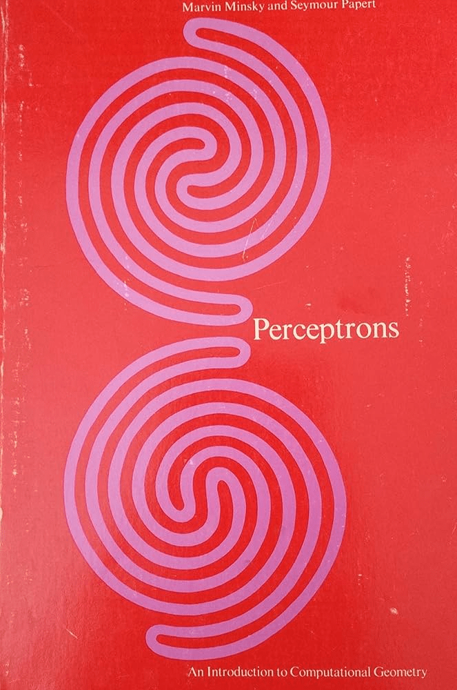
Minsky & Papert
Perceptrons, 1969
\(\underbrace{\quad\qquad\qquad}_{\vec x}\)
\(\underbrace{\qquad}_{h_{\vec w}}\)
\({\vec w}\)
\(\underbrace{\qquad}\)
updates
with \(\vec y\)
\(\underbrace{\qquad}\)
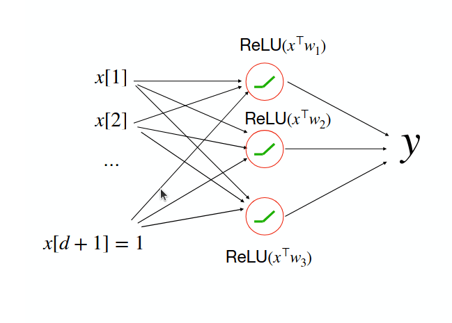
No good algorithm for multiple layers (yet)
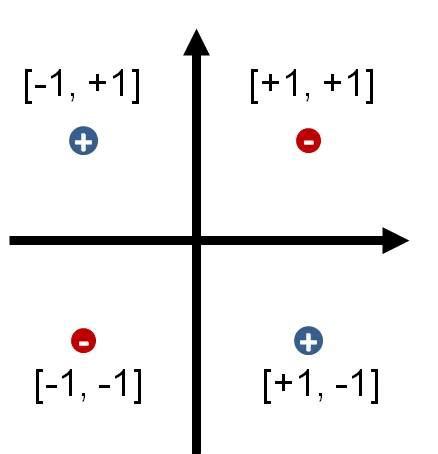
Fundamental limitations of linear classifiers (XOR)
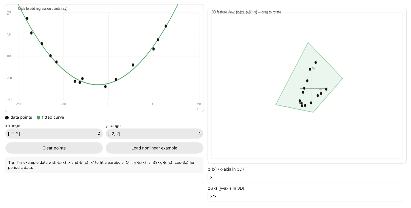
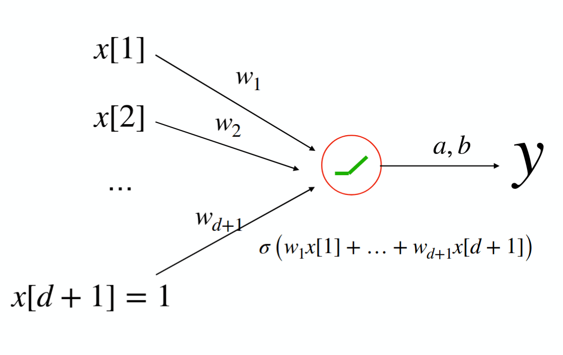
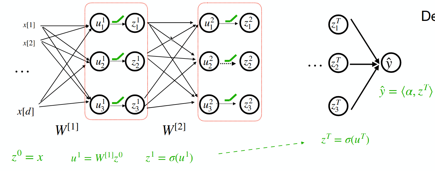
$$z = w x, \quad h = \sigma(z),\quad \hat{y} = a \cdot h + b,\quad \ell(\hat y, y)=(y-\hat y)^2$$
What are \( \frac{\partial \ell}{\partial w}\), \(\frac{\partial \ell}{\partial a}\), \(\frac{\partial \ell}{\partial b}\)?
By Sarah Dean


