

Sarah Dean PRO
asst prof in CS at Cornell
(down arrow for handout slides)
\(\mathbf x = \)[Yes, Game of Thrones, No, Souvlaki House, 9] ?
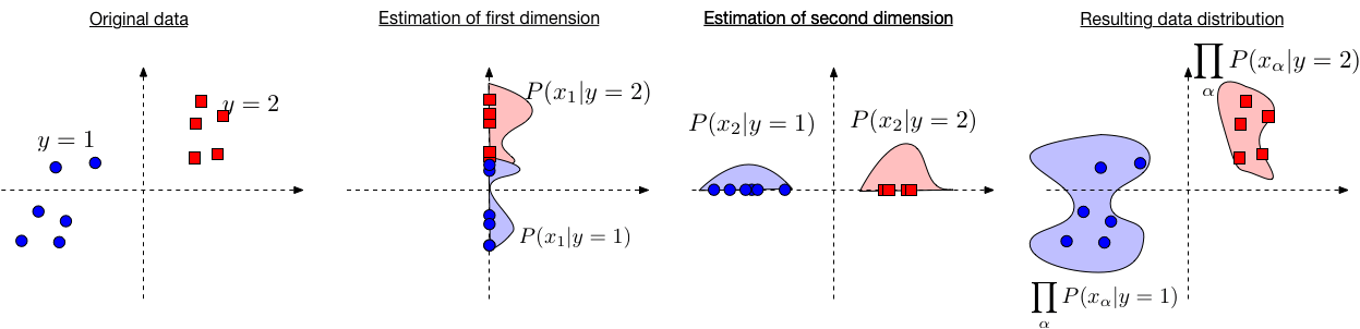
$$ \begin{align} h(\mathbf{x}) &= \operatorname*{argmax}_y P(y|\mathbf{x}) \\ &= \operatorname*{argmax}_y \frac{P(\mathbf{x}|y)P(y)}{P(\mathbf{x})} \\ &= \operatorname*{argmax}_y P(\mathbf{x}|y)P(y) \\ &= \operatorname*{argmax}_y \textstyle \prod_{\alpha=1}^d P(x_\alpha|y) P(y) \\ &= \operatorname*{argmax}_y \textstyle \sum_{\alpha=1}^d \log(P(x_\alpha|y)) + \log(P(y)) \end{align} $$
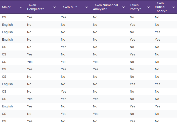
Example: \(\mathbf x=\) electives taken, \(y=\) major
P(ML=Y | Major=CS) \(\approx [\hat \theta_{Y,CS}]_{ML} = \frac{9}{10}\)
P(Major=CS) \(\approx\)
\( \hat \pi_{CS} = \frac{10}{15}\)
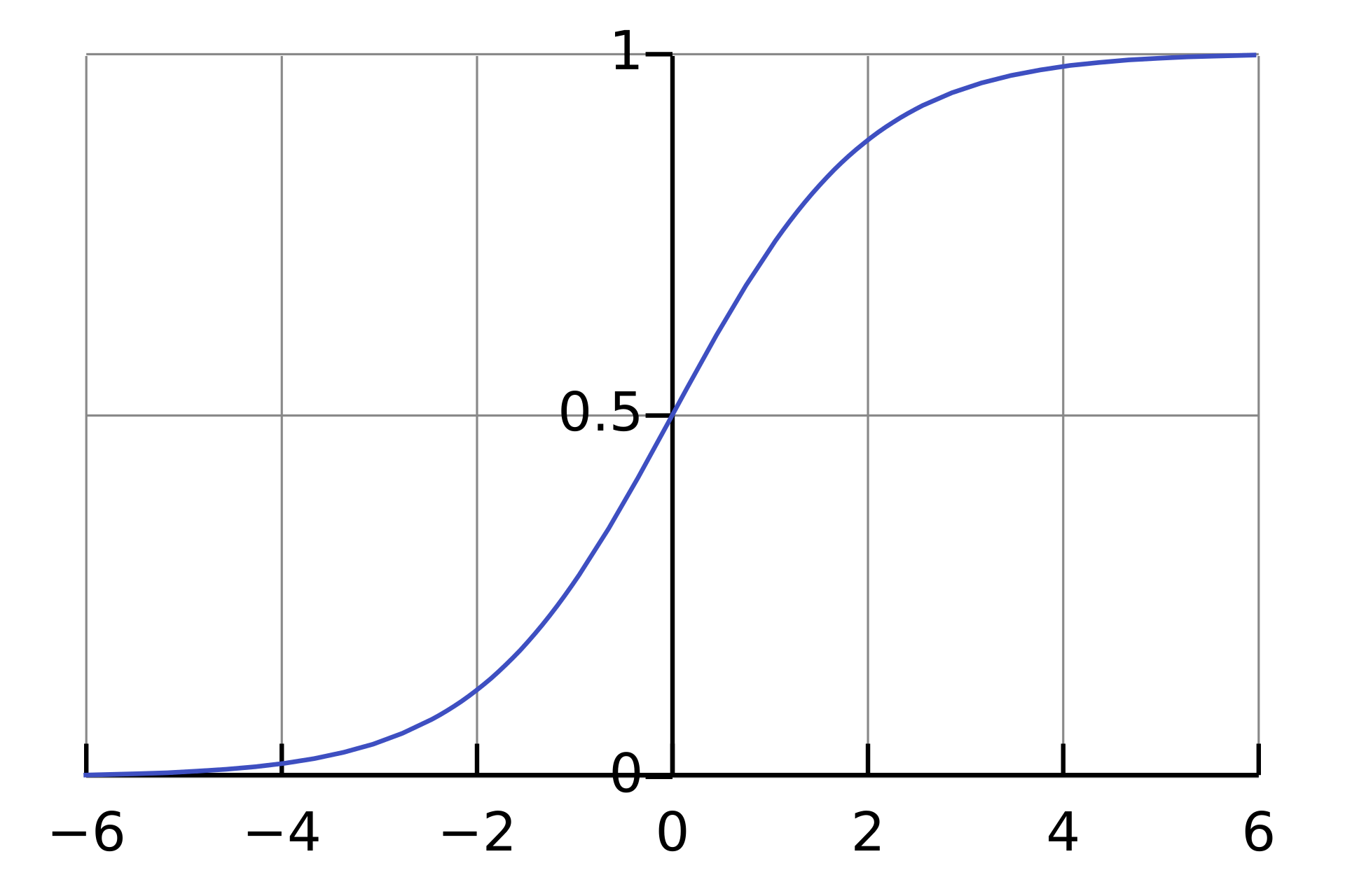
$$f(u) = \frac{1}{1+\exp(-u)}$$
$$P(y|\mathbf x) = \frac{1}{1+\exp(-y( \mathbf w^\top \mathbf x+b) )}$$
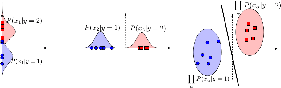
For many common cases, Naive Bayes produces a linear decision boundary!
$$ \begin{align} \log\left[P(\mathbf{x}|Y=+1)\right] &=\log\left[\Pi_{\alpha=1}^d P(x_\alpha | Y=+1) \right]\\ &=\sum_{\alpha=1}^d x_\alpha\log[\theta_{\alpha+}] \\ &=\sum_{\alpha=1}^d x_\alpha w^+_\alpha=\mathbf{x}^\top \mathbf{w}_+. \end{align} $$
$$\begin{align} P(Y=+1\ |\ \mathbf{x}) &=\frac{P(\mathbf{x} \ |\ Y= +1)P(Y=+1)}{P(\mathbf{x})}\\&= \frac{P(\mathbf{x} \ |\ Y= +1)P(Y=+1)}{P(\mathbf{x} \ |\ Y= +1)P(Y=+1)+P(\mathbf{x} \ |\ Y= -1)P(Y=-1)}\end{align}$$
$$\begin{align} P(Y=+1\ |\ \mathbf{x})=&\frac{P(\mathbf{x} \ |\ Y= +1)P(Y=+1)}{P(\mathbf{x} \ |\ Y= +1)P(Y=+1)+P(\mathbf{x} \ |\ Y= -1)P(Y=-1)}\\ &=\frac{e^{\mathbf{x}^\top \mathbf{w}_+}P(Y=+1)} {e^{\mathbf{x}^\top \mathbf{w}_+}P(Y=+1)+e^{\mathbf{x}^\top \mathbf{w}_-}P(Y=-1)}&\\ &=\frac{1}{1+e^{-\mathbf{x}^\top \mathbf{w}}\frac{P(Y=-1)}{P(Y=+1)} }\\ & =\frac{1}{1+e^{-(\mathbf{x}^\top \mathbf{w}+b)}} \ \ \ \end{align}$$
By Sarah Dean


