1. Setting: Linear Classifiers

• Question: Which separating hyperplane is the best? Can you draw a better one?
• 2D Interactive Demo

1. Setting: Linear Classifiers

• Data: \(y_i \in \{+1, -1\}\) (binary classification) and \(\mathbf x_i \in \mathbb{R}^d\)
• Model: Linear classifier \(h(\mathbf{x}) = \text{sign}(\mathbf{w}^\top\mathbf{x} + b)\)
• Idea: Use optimization to find the best separating hyperplane
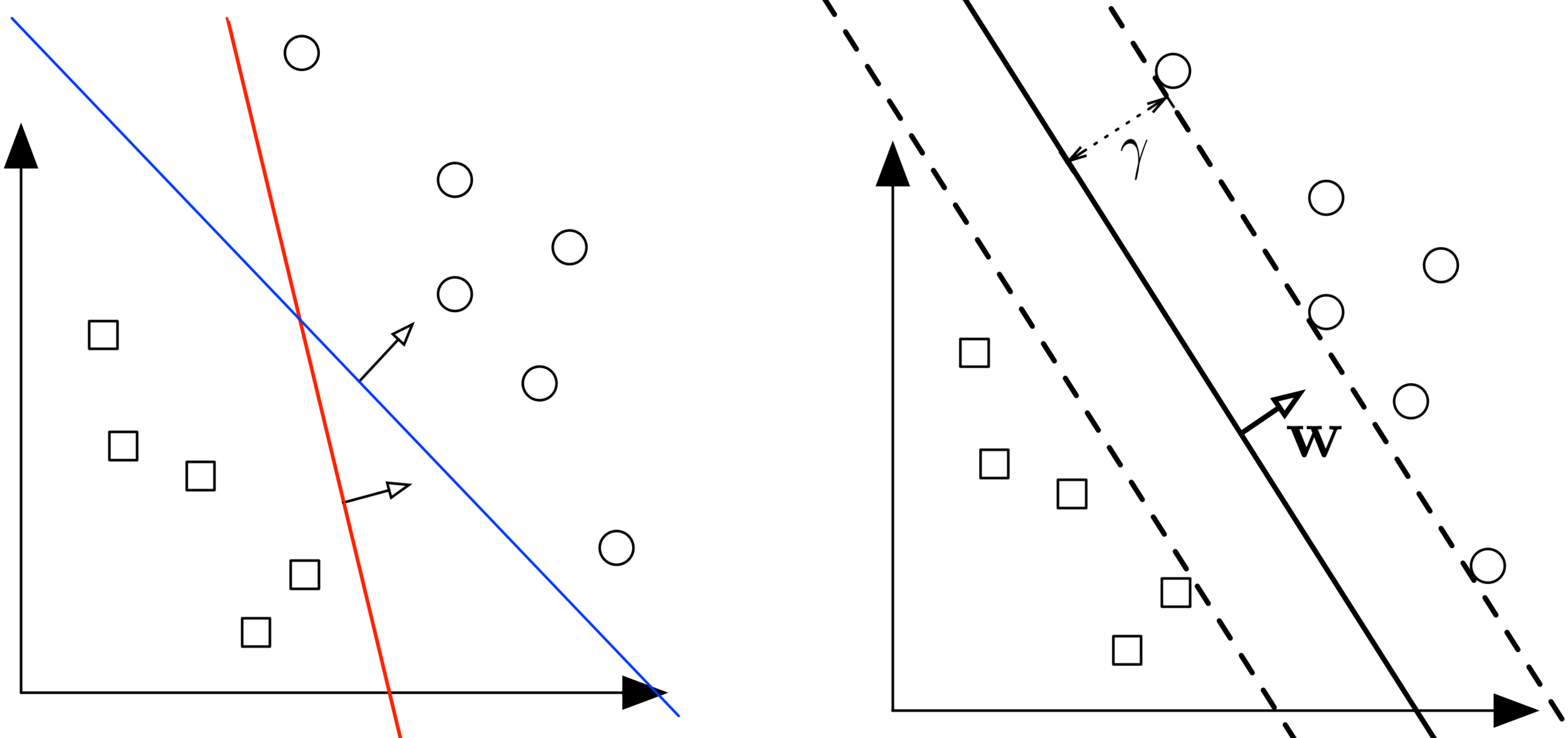
• Question: Which separating hyperplane is the best? Can you draw a better one?

2. Margin

2. Margin

• Decision boundary: is a hyperplane $$\mathcal{H} = \{\mathbf{x} : \mathbf{w}^\top\mathbf{x} + b = 0\}$$
• Scale invariance: a hyperplane with params \(\beta\mathbf{w}, \beta b\)
  is identical to that with parameters \(\mathbf{w}, b\) for all \(\beta \neq 0\)
• Margin (\(\gamma\)): Distance from hyperplane to closest point across both classes (recall Perceptron Lecture)

3. Derivation: Distance from Point to Hyperplane

3. Derivation: Distance from Point to Hyperplane

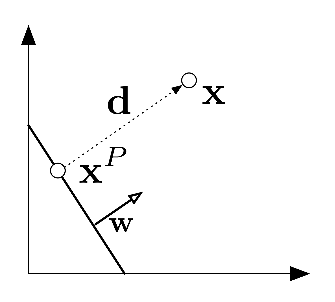
• Let \(\mathbf{d}\) = vector from \(\mathcal{H}\) to \(\mathbf{x}\) of minimum length,
  \(\mathbf{x}^P\) = projection of \(\mathbf{x}\) onto \(\mathcal{H}\)
• Fact 1: Relationship between points: \(\mathbf{x}^P + \mathbf{d}= \mathbf{x} \)
• Fact 2: Parallel vectors: \(\mathbf{d} = \alpha\mathbf{w}\) for some \( \alpha \in \mathbb{R}\)
• Fact 3: \(\mathbf{x}^P\) lies on the hyperplane: \(\mathbf{w}^\top\mathbf{x}^P + b = 0\)
• Substitute 1 and 2 into 3: $$0= \mathbf{w}^\top\mathbf{x}^P + b = \mathbf{w}^\top(\mathbf{x} - \mathbf{d}) + b = \mathbf{w}^\top(\mathbf{x} - \alpha\mathbf{w}) + b \\  \text{solve for }\alpha:\quad  \alpha = \frac{\mathbf{w}^\top\mathbf{x} + b}{\mathbf{w}^\top\mathbf{w}}$$
• Distance is therefore given by $$ \|\mathbf{d}\|_2 = |\alpha|\|\mathbf{w}\|_2 = \frac{|\mathbf{w}^\top\mathbf{x} + b|}{{\mathbf{w}^\top\mathbf{w}}} \|\mathbf w\|_2 = \frac{|\mathbf{w}^\top\mathbf{x} + b|}{\|\mathbf{w}\|_2} $$

4/5. Derivation: Hard Margin SVM

• Objective: Maximize margin while ensuring separating hyperplane $$ \operatorname*{argmax}_{\mathbf{w}, b} \frac{1}{\|\mathbf{w}\|_2} \min_{\mathbf{x}_i \in D} |\mathbf{w}^\top\mathbf{x}_i + b| \quad \text{s.t.} \quad \forall i: y_i(\mathbf{w}^\top\mathbf{x}_i + b) \geq 0 $$
• Question: Can you explain each of the following steps to your partner? Refer to your handout
  1. Fix the scale \(\min_{\mathbf{x} \in D} \|\mathbf{w}^\top\mathbf{x} + b\|_2 = 1\)
  2. New objective \(  \operatorname*{argmax}_{\mathbf{w}, b} \frac{1}{\|\mathbf{w}\|_2} = \operatorname*{argmin}_{\mathbf{w}, b} \|\mathbf{w}\|_2 = \operatorname*{argmin}_{\mathbf{w}, b} \mathbf{w}^\top\mathbf{w} \)
  3. New optimization problem: $$ \begin{align*} \min_{\mathbf{w}, b} \quad & \mathbf{w}^\top\mathbf{w} \\ \text{s.t.} \quad & \forall i: y_i(\mathbf{w}^\top\mathbf{x}_i + b) \geq 0 \\ & \min_i |\mathbf{w}^\top\mathbf{x}_i + b| = 1 \end{align*} $$
  4. Simplified final formulation: $$ \begin{align*} \min_{\mathbf{w}, b} \quad & \mathbf{w}^\top\mathbf{w} \\ \text{s.t.} \quad & \forall i: y_i(\mathbf{w}^\top\mathbf{x}_i + b) \geq 1 \end{align*} $$

4. Max Margin Classifier: Initial Formulation

• Margin: Minimum distance from data point \(\mathbf{x}\) to hyperplane \(\mathcal{H}\) $$ \gamma(\mathbf{w}, b) = \min_{\mathbf{x} \in D} \frac{|\mathbf{w}^\top\mathbf{x} + b|}{\|\mathbf{w}\|_2} $$
• Objective: Maximize margin while ensuring separating hyperplane $$ \operatorname*{argmax}_{\mathbf{w}, b} \frac{1}{\|\mathbf{w}\|_2} \min_{\mathbf{x}_i \in D} |\mathbf{w}^\top\mathbf{x}_i + b| \quad \text{s.t.} \quad \forall i: y_i(\mathbf{w}^\top\mathbf{x}_i + b) \geq 0 $$
• Simplification: Hyperplane is scale invariant, so fix the scale to $$\min_{\mathbf{x} \in D} \|\mathbf{w}^\top\mathbf{x} + b\|_2 = 1$$ $$ \operatorname*{argmax}_{\mathbf{w}, b} \frac{1}{\|\mathbf{w}\|_2} \cdot 1 = \operatorname*{argmax}_{\mathbf{w}, b} \frac{1}{\|\mathbf{w}\|_2} = \operatorname*{argmin}_{\mathbf{w}, b} \|\mathbf{w}\|_2 = \operatorname*{argmin}_{\mathbf{w}, b} \mathbf{w}^\top\mathbf{w} $$
• New optimization problem: $$ \begin{align*} \min_{\mathbf{w}, b} \quad & \mathbf{w}^\top\mathbf{w} \\ \text{s.t.} \quad & \forall i: y_i(\mathbf{w}^\top\mathbf{x}_i + b) \geq 0 \\ & \min_i |\mathbf{w}^\top\mathbf{x}_i + b| = 1 \end{align*} $$

5. Hard-Margin SVM

• Constraints ensure \(y_i(\mathbf{w}^\top\mathbf{x}_i + b) \geq 0\) and \(|\mathbf{w}^\top\mathbf{x}_i + b| \geq 1\), which is equivalent to a combined constraint \(y_i(\mathbf{w}^\top\mathbf{x}_i + b) \geq 1\) since \(y_i=\pm 1\)
• Final formulation: equivalent to previous slide but simpler $$ \begin{align*} \min_{\mathbf{w}, b} \quad & \mathbf{w}^\top\mathbf{w} \\ \text{s.t.} \quad & \forall i: y_i(\mathbf{w}^\top\mathbf{x}_i + b) \geq 1 \end{align*} $$
• Objective is quadratic, constraints are linear, so can be solved efficiently with any quadratic program optimization solver
• Unique solution whenever a separating hyperplane exists, infeasible (solver error) if data is not linearly separable
• Interpretation: Find the "simplest" hyperplane (smaller \(\mathbf{w}^\top\mathbf{w}\)) such that all data lies at least 1 unit away from the hyperplane on the correct side

6. Support Vectors

6. Support Vectors

• Definition: For optimal \((\mathbf{w}, b)\), training points with tight constraints: $$ y_i(\mathbf{w}^\top\mathbf{x}_i + b) = 1 $$
• They must exist: if all training points had strict inequality (\(>\)), we could scale down \((\mathbf{w}, b)\) to get lower objective value.
• Importance:
  • Define the maximum margin of the hyperplane
  • Determine the direction of the hyperplane
  • Moving a support vector changes the resulting hyperplane
  • Other data points (far from boundary) don't affect the solution

7. Derivation: Soft-Margin SVM

7. Slack Variables

• What if data is not linearly separable?
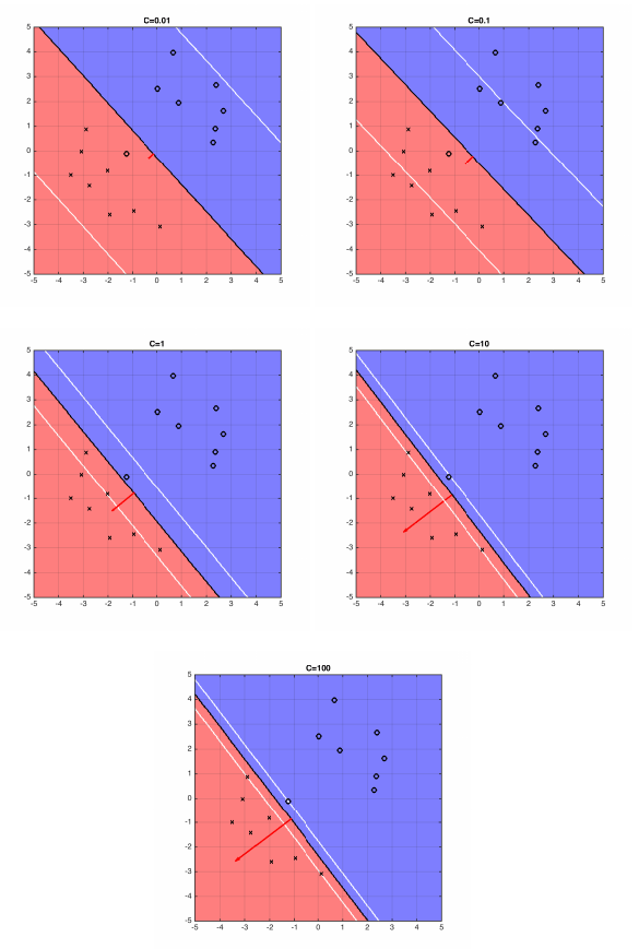
• Solution: Allow constraints to be violated slightly with slack variables \(\xi_i\) allowing \(\mathbf{x}_i\) to be closer to hyperplane (or even on wrong side), but with penalty in objective $$ \begin{align*} \min_{\mathbf{w}, b, \boldsymbol{\xi}} \quad & \mathbf{w}^\top\mathbf{w} + C\sum_{i=1}^n \xi_i \\ \text{s.t.} \quad & \forall i: y_i(\mathbf{w}^\top\mathbf{x}_i + b) \geq 1 - \xi_i \\ & \forall i: \xi_i \geq 0 \end{align*} $$
• For larger values of \(C\), SVM becomes very strict and small violations heavily penalized. For smaller values, may "sacrifice" some points to obtain simpler solution (lower \(\|\mathbf{w}\|_2^2\)).

8. Soft-Margin SVM

• For \(C \neq 0\), objective minimizes \(\xi_i\), so constraint holds as equality: $$ \xi_i = \begin{cases} 1 - y_i(\mathbf{w}^\top\mathbf{x}_i + b) & \text{if } y_i(\mathbf{w}^\top\mathbf{x}_i + b) < 1 \\ 0 & \text{if } y_i(\mathbf{w}^\top\mathbf{x}_i + b) \geq 1 \end{cases} $$
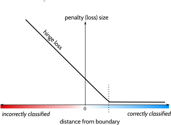
• Equivalent to the one line expression $$ \xi_i = \max(1 - y_i(\mathbf{w}^\top\mathbf{x}_i + b), 0) $$
• Hinge Loss Formulation: gives unconstrained version: $$ \min_{\mathbf{w}, b} \underbrace{\mathbf{w}^\top\mathbf{w}}_{\ell_2\text{-regularizer}} + C\sum_{i=1}^n \underbrace{\max[1 - y_i(\mathbf{w}^\top\mathbf{x}_i + b), 0]}_{\text{hinge-loss}} $$
• Interpretation: Balance "simplicity" of hyperplane against ensuring all data lies on correct side with a distance of 1
• Gradient descent (or related methods) are possible 

8. Hinge Loss and Gradient

8. Hinge Loss Gradient

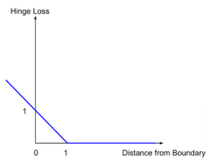
• Scalar hinge: \(h(u) = \max(0, 1-u)\) penalizes \(u\) (\(= y_i(\mathbf{w}^\top \mathbf{x}_i + b)\)) within the margin (including misclassified), zero loss when \(u \geq 1\)
• Hinge is non-differentiable at \(t = 1\), so we use a subderivative (not unique): $$\frac{d}{d u} h(u) = \begin{cases} -1 & t < 1 \\ 0 & t > 1 \\ \text{any value in }[-1,0] & t=1\end{cases}$$

• Using chain rule, \(\nabla_{\textbf w} h( y_i(\mathbf{w}^\top \mathbf{x}_i + b)= y_i \mathbf{x}_i \cdot \mathbf{1}[y_i(\mathbf{w}^\top \mathbf{x}_i + b) < 1] \) (we pick \(0\) subderivative for convenience)
• The overall gradient is $$ \nabla_{\mathbf{w}}\mathcal L(\mathbf w, b) = 2\mathbf{w} - C \sum_{i=1}^{n} y_i \mathbf{x}_i \cdot \mathbf{1}[y_i(\mathbf{w}^\top \mathbf{x}_i + b) < 1] \\ \nabla_{\mathbf{b}}\mathcal L(\mathbf w, b) = -C \sum_{i=1}^{n} y_i \cdot \mathbf{1}[y_i(\mathbf{w}^\top \mathbf{x}_i + b) < 1] $$