\text{Gradient, } \nabla
\text{in higer dimesions}
\text{let us define a vector quantity as follows:}
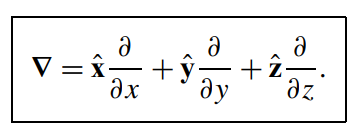
\text{We start first by defining the operator \textcolor{red}{Nabla } } \color{red}{\nabla}:
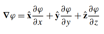
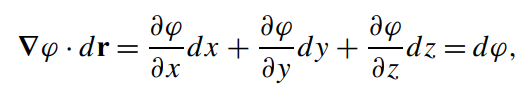
\text{The application of this \textcolor{orange}{operator} on a \textcolor{red}{scalar function} gives us:}
\displaystyle d\varphi(x,y,z)=\frac{\partial \varphi}{\partial x} dx+\frac{\partial \varphi}{\partial y} dy+\frac{\partial \varphi}{\partial z} dz
\text{To provide a motivation for the vector nature of partial derivatives, we }
\text{introduce the \textbf{the total variation of a function} }F(x,y)
\displaystyle d F=\frac{\partial F}{\partial x} dx+\frac{\partial F}{\partial y} dy
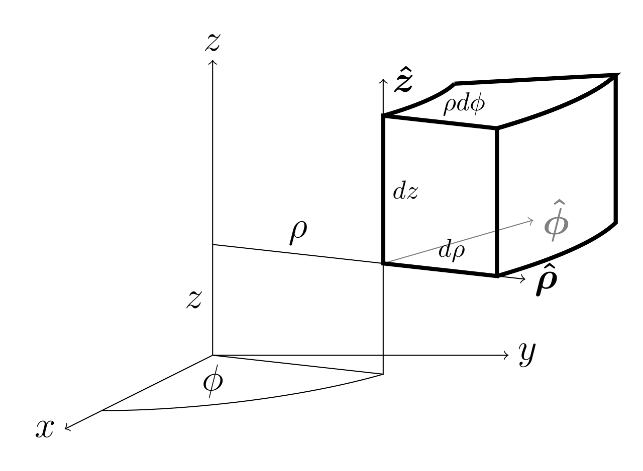
\Big(\displaystyle \frac{\partial }{\partial r}\hat{r} +\frac{\partial }{\partial z}\hat{z}+\frac{1}{r}\frac{\partial}{\partial \varphi}\hat{\varphi} \Big)
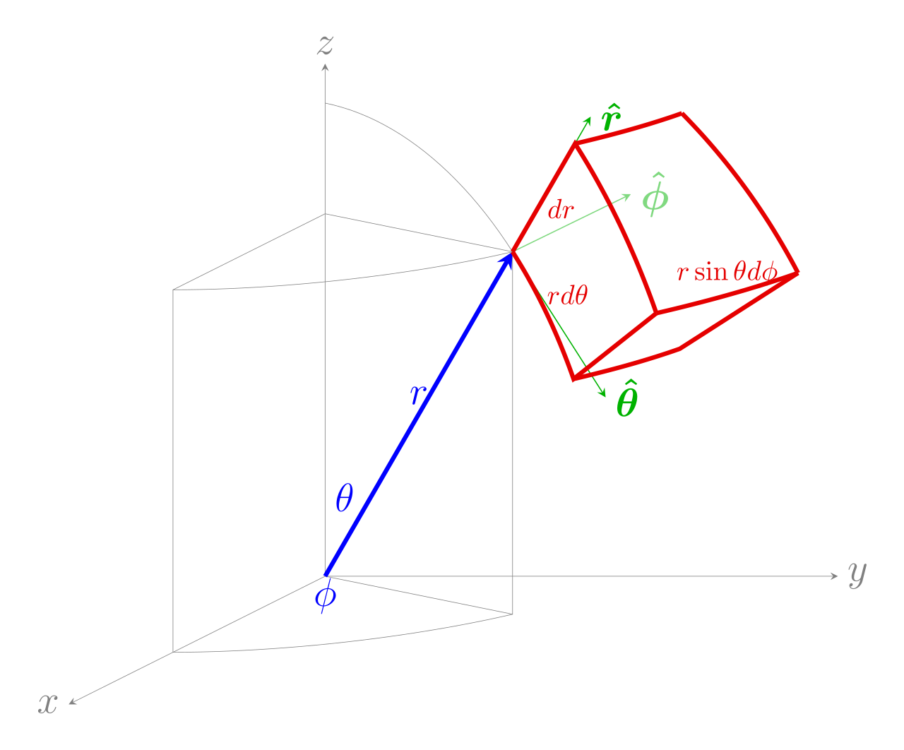
\Big(\displaystyle \frac{\partial }{\partial r}\hat{r} +\frac{1}{r}\frac{\partial }{\partial \theta}\hat{\theta}+\frac{1}{r \sin\theta}\frac{\partial}{\partial \varphi}\hat{\varphi} \Big)
\text{Spherical coordinates}
\text{Cylindrical coordinates}
\text{with these definitions, the \textcolor{orange}{total variation} of a function can be expressed straightforwardly}
\text{Where}
\text{consider P and Q to be two points on a surface }\varphi(x,y,z)=C, \text{ a constant}
d\textbf{r}=\hat{\textbf{x}} dx+\hat{\textbf{y}} dy+\hat{\textbf{z}} dz
d\varphi=(\mathbf{\nabla}\varphi).d\mathbf{r}=0
\text{\textcolor{red}{Remark:} }
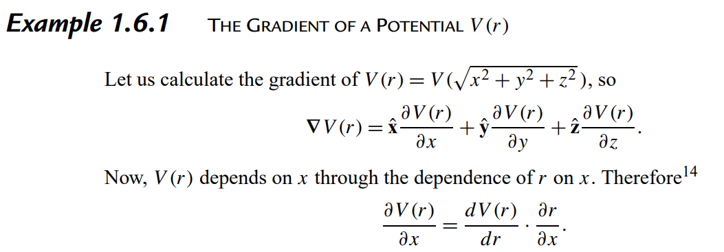
\text{This is valid for a potential } V(r) \text{ \textcolor{orange}{depending on r only }and not on the angles}
\displaystyle V(r)=-\frac{1}{r}
\text{Example:}
\displaystyle \nabla V(r)=\frac{1}{r^2} \hat{r}
\begin{aligned}
\nabla V(r) & =(\hat{\mathbf{x}} x+\hat{\mathbf{y}} y+\hat{\mathbf{z}} z) \frac{1}{r} \frac{d V}{d r} \\
& =\frac{\mathbf{r}}{r} \frac{d V}{d r}=\hat{\mathbf{r}} \frac{d V}{d r}
\end{aligned}
\text{Permuting the coordinates }(x\rightarrow y, y\rightarrow z,z\rightarrow x) \text{ to obtain } y \text{ and } z\text{ derivatives, we get}
\text{Divergence}
\text{The application of the operator \textcolor{red}{Nabla ∇}on a \textcolor{green}{vector} will give you the divergence}
\displaystyle \nabla .\mathbf{V} =\frac{\partial V_x}{\partial x}+\frac{\partial V_y}{\partial y}+\frac{\partial V_z}{\partial z}
\begin{aligned}
\boldsymbol{\nabla} \cdot \mathbf{r} & =\left(\hat{\mathbf{x}} \frac{\partial}{\partial x}+\hat{\mathbf{y}} \frac{\partial}{\partial y}+\hat{\mathbf{z}} \frac{\partial}{\partial z}\right) \cdot(\hat{\mathbf{x}} x+\hat{\mathbf{y}} y+\hat{\mathbf{z}} z) \\
& =\frac{\partial x}{\partial x}+\frac{\partial y}{\partial y}+\frac{\partial z}{\partial z}
\end{aligned}
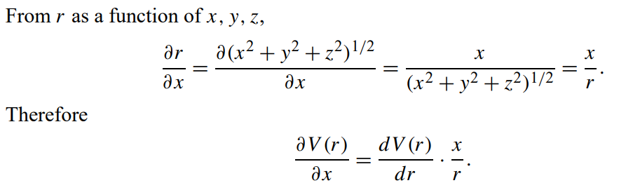
\text { \bf{Example 1.7.1}: \textcolor{red}{Divergence of Coordinate Vector }}
\text{Calculate $\boldsymbol{\nabla} \cdot \mathbf{r}$ :}
\boldsymbol{\nabla} \cdot \mathbf{r}=3.
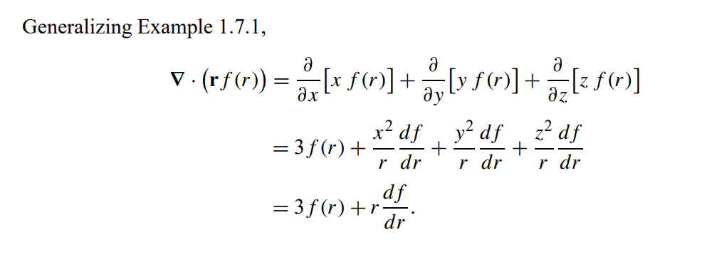
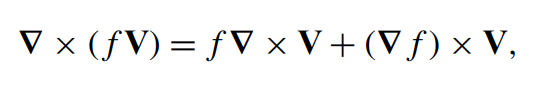
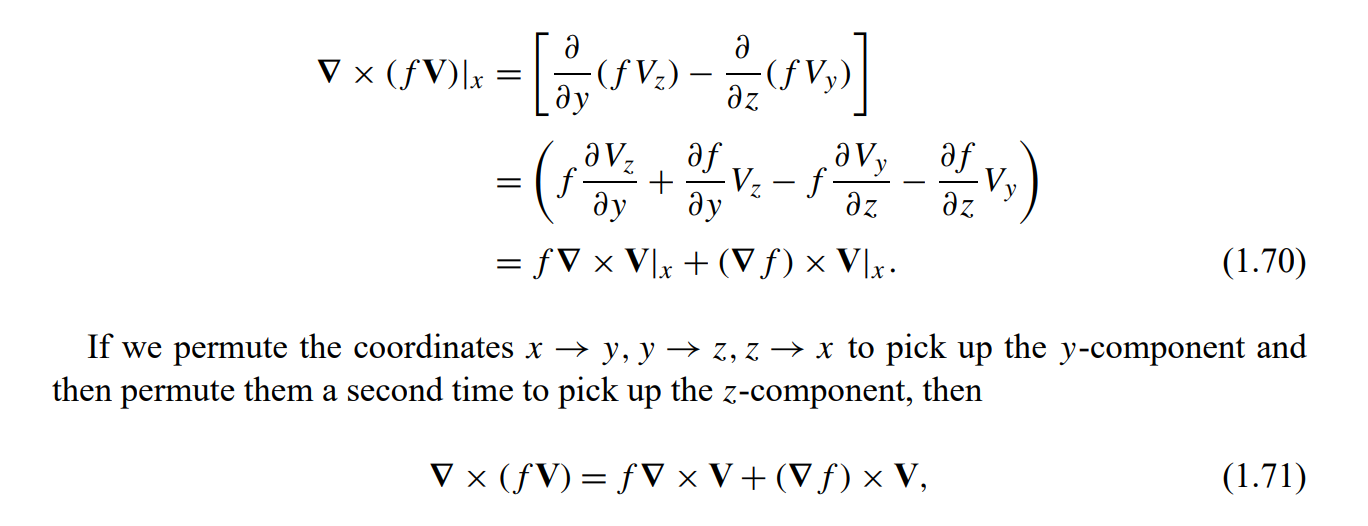
\text{The combination $\boldsymbol{\nabla} \cdot(f \mathbf{V})$, in which $f$ is a scalar function and $\mathbf{V}$ is a vector function, may }
\text{be written}
\begin{aligned}
\boldsymbol{\nabla} \cdot(f \mathbf{V}) & =\frac{\partial}{\partial x}\left(f V_x\right)+\frac{\partial}{\partial y}\left(f V_y\right)+\frac{\partial}{\partial z}\left(f V_z\right) \\
& =\frac{\partial f}{\partial x} V_x+f \frac{\partial V_x}{\partial x}+\frac{\partial f}{\partial y} V_y+f \frac{\partial V_y}{\partial y}+\frac{\partial f}{\partial z} V_z+f \frac{\partial V_z}{\partial z} \\
& =(\boldsymbol{\nabla} f) \cdot \mathbf{V}+f \boldsymbol{\nabla} \cdot \mathbf{V}
\end{aligned}
\boldsymbol{\nabla} \cdot(f \mathbf{V})=(\boldsymbol{\nabla} f) \cdot \mathbf{V}+f \boldsymbol{\nabla} \cdot \mathbf{V}
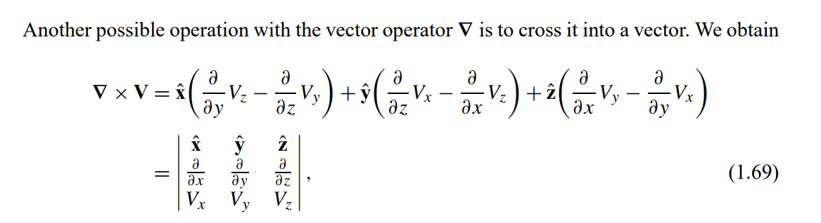
\text{Curl,} \nabla \times
\text{Solution:}
\text{Prove that:}
\text{Suppose that the force is: } \displaystyle \bold{F}(\bold{r})=\bold{\hat{r}} f(r)\\
\text{We used the fact that } \hat{r}\times \hat{r}=0 \text{ and the fact that f(r) } \text{doesn't depend on } \theta \text{ or } \varphi\\
\text{\textcolor{red}{Question:} Find the Curl for a radial force.}
\text{Hint: use equation 1.71 or any other method}
\text{In the spherical coordinates, we can write:}\\
\Big(\displaystyle \frac{\partial }{\partial r}\hat{r} +\frac{1}{r}\frac{\partial }{\partial \theta}\hat{\theta}+\frac{1}{r \sin\theta}\frac{\partial}{\partial \varphi}\hat{\varphi} \Big)
\times \hat{r} f(r)=0
\text{SUCCESSIVE APPLICATIONS OF }\nabla
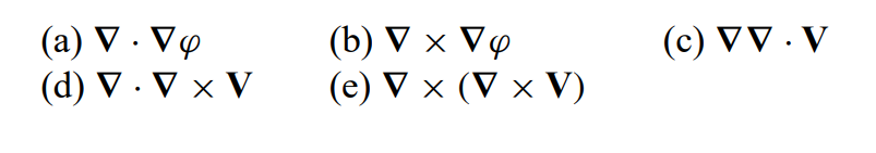
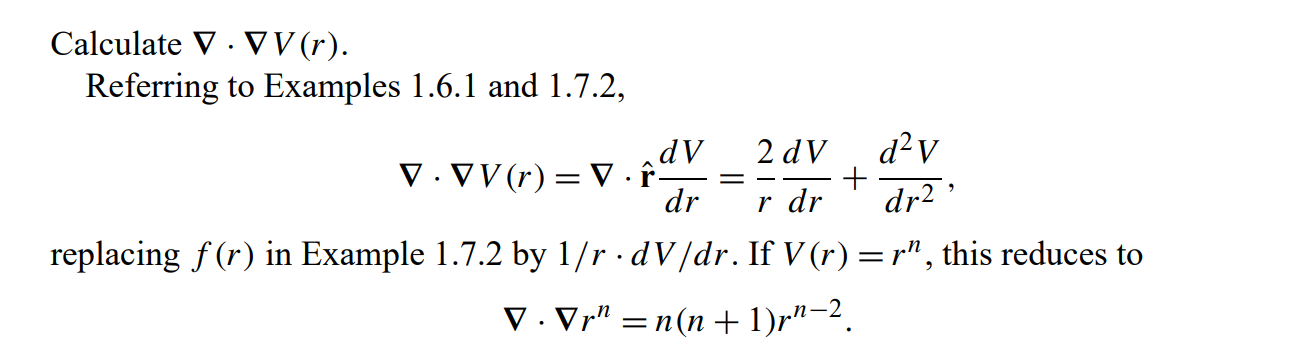
\text{a) Laplacian}
b)
\begin{aligned}
\nabla \times \nabla \varphi= & \hat{\mathbf{x}}\left(\frac{\partial^2 \varphi}{\partial y \partial z}-\frac{\partial^2 \varphi}{\partial z \partial y}\right)+\hat{\mathbf{y}}\left(\frac{\partial^2 \varphi}{\partial z \partial x}-\frac{\partial^2 \varphi}{\partial x \partial z}\right) \\
& +\hat{\mathbf{z}}\left(\frac{\partial^2 \varphi}{\partial x \partial y}-\frac{\partial^2 \varphi}{\partial y \partial x}\right)=0,
\end{aligned}
\begin{aligned}
\boldsymbol{\nabla} \cdot \boldsymbol{\nabla} \varphi & =\left(\hat{\mathbf{x}} \frac{\partial}{\partial x}+\hat{\mathbf{y}} \frac{\partial}{\partial y}+\hat{\mathbf{z}} \frac{\partial}{\partial z}\right) \cdot\left(\hat{\mathbf{x}} \frac{\partial \varphi}{\partial x}+\hat{\mathbf{y}} \frac{\partial \varphi}{\partial y}+\hat{\mathbf{z}} \frac{\partial \varphi}{\partial z}\right) \\
& =\frac{\partial^2 \varphi}{\partial x^2}+\frac{\partial^2 \varphi}{\partial y^2}+\frac{\partial^2 \varphi}{\partial z^2}
\end{aligned}
\boldsymbol{\nabla} \cdot \boldsymbol{\nabla} \times \mathbf{V}=0
\boldsymbol{\nabla} \times(\boldsymbol{\nabla} \times \mathbf{V})=\nabla \nabla \cdot \mathbf{V}-\boldsymbol{\nabla} \cdot \boldsymbol{\nabla} \mathbf{V},
\text{Useful relations:}
\text{Non trivial calculation rules:}
\begin{aligned}
& \operatorname{div} \operatorname{grad} f \equiv \nabla \cdot \nabla f \equiv \nabla^2 f \\
& \operatorname{curl} \operatorname{grad} f \equiv \nabla \times \nabla f=\mathbf{0} \\
& \operatorname{div} \operatorname{curl} \mathbf{A} \equiv \nabla \cdot(\nabla \times \mathbf{A})=0 \\
& \operatorname{curl} \operatorname{curl} \mathbf{A} \equiv \nabla \times(\nabla \times \mathbf{A})=\nabla(\nabla \cdot \mathbf{A})-\nabla^2 \mathbf{A} \\
& \nabla^2(f g)=f \nabla^2 g+2 \nabla f \cdot \nabla g+g \nabla^2 f
\end{aligned}
\text{Magnetic field and gauge transformation}
\text{The solution to the homogenious Maxwell equations are}
\text{The solution is not unique: if we do the transformation}
\text{However, the electric field becomes}
\text{That is why, we conclude that the additional transformation}
\text{Will leave both E and B unchanged}
\text{A particular choice of the scalar and vector potentials is a gauge }
\displaystyle \varphi\rightarrow\varphi-\frac{\partial \psi}{\partial t}
\displaystyle \mathbf{E}=-\nabla\varphi-\frac{\partial \mathbf{A}}{\partial t}, \hspace{5mm}\mathbf{B}=\nabla\times \mathbf{A}
\mathbf{A}\rightarrow\mathbf{A}+\nabla\psi
\text{B remains the same because }\nabla\times\nabla \psi=0
\mathbf{B}=\nabla\times(\mathbf{A}+\nabla \psi)=\nabla\times \mathbf{A}
\displaystyle \mathbf{E}=-\nabla\Big(\varphi+\frac{\partial \psi}{\partial t}\Big)-\frac{\partial \mathbf{A}}{\partial t}
\displaystyle \partial V \text{ is the closed surface englobing the volume }V
\text{Let } \bold{V} \text{ be the vector representing the electric field } \bold{E}(x,y,z)\\
\text{From Maxwell equations, we have } \displaystyle \nabla \bold{E}=\frac{\rho}{\epsilon_0}
\text{We deduce at the end that} \displaystyle \iint_{\partial V} \bold{E} d\bm{ \sigma}=\frac{Q_{\text{enclosed}}}{\epsilon_0}
\text{This is the Gauss Law we studied in phys 102}
\text{Example 1:}
\text{It relies the flux of a vector field through a closed surface to the divergence}
\text{of the field in the \textcolor{red}{closed }volume}
\text{Gauss-Ostrogradski theorem}
\displaystyle \iint_{\partial V} \bold{E} \hspace{1mm} d\bm{ \sigma}=\iiint_V \nabla \bold{E }\hspace{1mm} dV
\displaystyle \oiint_{\partial V} \bold{V} .\hspace{1mm}d \bm{\sigma}=\iiint_V \nabla .\mathbf{V} d\tau
\text{(Divergence theorem)}
\displaystyle \int_C \overrightarrow {F} d\vec{r}=\iint_D (\vec{\nabla} \times \vec{F}) d\vec{A}
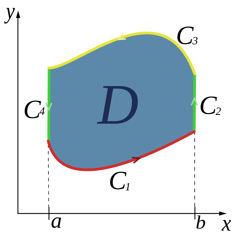
\text{Green's theorem}
\text{It relies the line integral of a vector over a closed curve to the integral of}
\text{the curl of the vector over the area of the curve domain}
\text{another form of this reads:}
\text{The \textcolor{red}{line C }is defined \textcolor{red}{anticlockwise}}
\displaystyle
\oint_c (P dx+Qdy)=\iint_D \Big(\frac{\partial P}{\partial x}-\frac{\partial Q}{\partial y}\Big)dx dy
\text{Solve $\oint_c y^3 d x-x^3 d y$ where C is a circle of radius 2 centered in origin.}
\text{Question:}
\text{Solve $\oint_c y^3 d x-x^3 d y$ where C is a circle of radius 2 centered in origin.}
\text{Question:}
\text{Identify $P$ and $Q$ from the line integral. Here, $P=y^3$ and $Q=-x^3$}
\begin{aligned}
& \oint_C y^3 d x-x^3 d y=\iint_D-3 x^2-3 y^2 d A \\
& =-3 \int_0^{2 \pi} \int_0^2 r^3 d r d \theta \\
& =-3 \int_0^{2 \pi} \frac{1}{4}\left[r^4\right]_0^2 d \theta \\
& =-3 \int_0^{2 \pi} 4 d \theta =-24 \pi
\end{aligned}
\text { Therefore, } \oint_c y^3 d x-x^3 d y=-24 \pi
\text{Stokes's theorem}
\text{Stokes theorem is the generalization of the Green's theorem to 3D}
\text{In other words, if you take the 3-dimensional formulation of Stokes' theorem}
\displaystyle \oint_{\partial \Sigma}\Big(F_x dx+F_y dy+F_z dz\Big)=
=\displaystyle \iint_\Sigma\bigg( \frac{\partial F_z}{\partial y}-\frac{\partial F_y}{\partial z}\bigg)dy dz+
\bigg( \frac{\partial F_x}{\partial z}-\frac{\partial F_z}{\partial x}\bigg)dz dx+
\bigg( \frac{\partial F_y}{\partial x}-\frac{\partial F_x}{\partial y}\bigg)dx dy
\text{and set, let's say, } F_z=0 \text{ and }dz=0. \text{The whole thing simplifies to}
\displaystyle \oint_{\partial \Sigma}\Big(F_x dx+F_y dy\Big)=\displaystyle \iint_\Sigma\bigg( \frac{\partial F_y}{\partial x}-\frac{\partial F_x}{\partial y}\bigg)dx dy
\text{Which is exactly the statement of the Green's theorem}
\displaystyle \oint \mathbf{V} \cdot d \bm{\lambda}=\int_S \nabla \times \mathbf{V} \cdot d \bm{\sigma}
\text{Problems:}
\displaystyle \oiint_S d \bm{\sigma}=0
\text{Using Gauss' theorem, prove that}
\text{if } S=\partial V, \text{ is a closed surface}
1.11.1
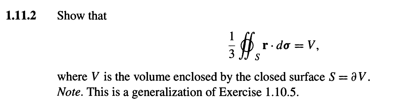
\oiint_S \mathbf{B} \cdot d \boldsymbol{\sigma}=\mathbf{0}
\text { for any closed surface } S \text {. }
\text { 1.11.3 \hspace{2cm} If } \mathbf{B}=\nabla \times \mathbf{A} \text {, show that }
% requires \usepackage{xcolor} % for colored words
% (optional) \usepackage{esint} % for \oiint (closed surface integral). Otherwise use \iint.
\begin{align*}
& \text{Suppose we wish to evaluate }\\
& \hspace{3cm} \iint_{S} \mathbf{F}\!\cdot\!\mathbf{n}\, dS, \\[0.4em]
& \text{where } S \text{ is the } \textcolor{blue}{\text{unit sphere}} \text{ defined by }\\
& \qquad S=\{(x,y,z)\in \mathbb{R}^{3} : x^{2}+y^{2}+z^{2}=1\},\\[0.4em]
& \text{and } \mathbf{F} \text{ is the } \textcolor{blue}{\text{vector field}} \\[0.2em]
& \qquad \mathbf{F}=2x\,\mathbf{i} + y^{2}\,\mathbf{j} + z^{2}\,\mathbf{k}.
\end{align*}
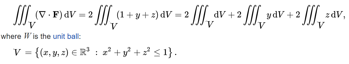
\text{Using the Gauss-Ostrogradsky theorem, we get}
\iiint_V y \mathrm{~d} V=\iiint_V z \mathrm{~d} V=0
\text { because the unit ball } V \text { has volume } \frac{4 \pi}{3} \text {. }
\oiint_S \mathbf{F} \cdot \mathbf{n} \mathrm{~d} S=2 \iiint_W d V=\frac{8 \pi}{3}
\text{Therfore,}
\begin{align*}
& \textit{1.12.1}\ \ \text{Given a vector } \mathbf{t}=-\hat{\mathbf{x}}\,y+\hat{\mathbf{y}}\,x, \text{ show, with the help of Stokes' theorem,}\\
& \text{that the integral around a continuous closed curve in the $xy$-plane}\\[0.3em]
& \hspace{3cm}\frac{1}{2}\oint \mathbf{t}\cdot d\boldsymbol{\lambda}
\;=\; \frac{1}{2}\oint \bigl(x\,dy-y\,dx\bigr)\;=\;A,\\[0.3em]
& \text{the area enclosed by the curve.}
\end{align*}
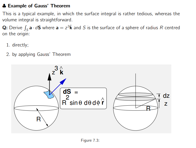
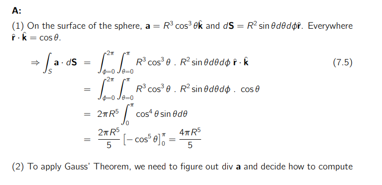
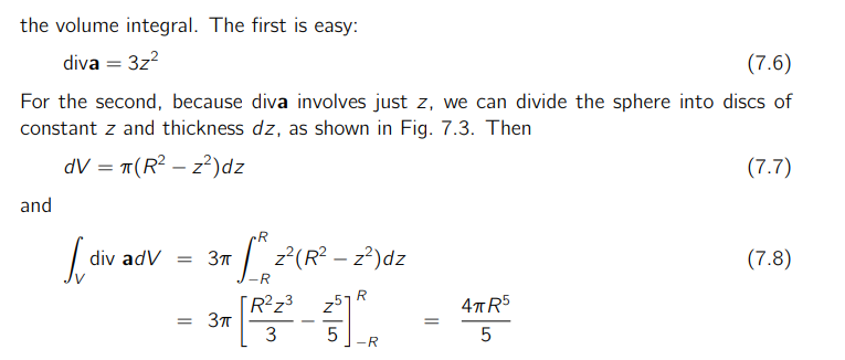
\text{Calculate the following integral over the surface S: } \displaystyle \iint_S \vec{a} \hspace{1mm}d\vec{S}
\text{S is the surface of a sphere of radius R. } \vec{a}=z^3 \hat{z}.\\
Gauss and Green theorems
By smstry


