COMP3010: Algorithm Theory and Design
Daniel Sutantyo, Department of Computing, Macquarie University
11.2 - Reduction
Where Are We Now?
11.2 - Reduction
\(\text{EXP}\)
\(\text{P}\)
\(\text{NP}\)
\(\text{EXP}\)
\(\text{NP-hard}\)
\(\text{NP-complete}\)
Where Are We Now
11.2 - Reduction
- NP-complete decision problems:
- NP-hard : any problem in NP can be reduced to it
- NP : we can verify if a solution is correct in P time
- Reduction
- converting one problem into another problem
- if I have two problems, A and B, and I can convert from A to B, and I can solve B, then:
- I can solve A using B
- I can argue that B is as hard as A
Reduction
11.2 - Reduction
Input for Problem A
Input for Problem B
Solution for Problem B
Solution for Problem A
REDUCER
REDUCER
SOLVER for B
Reduction (Decision Problem)
11.2 - Reduction
Input for Problem A
REDUCER
Input for Problem B
SOLVER for B
Yes / No
Point 1: I Can Solve A using B
11.2 - Reduction
- NP-complete problems are the most important class for proving or disproving P = NP because every problem in NP can be reduced to a problem in NP-complete
- So if just one problem in NP-complete can be done in polynomial time, that means we can solve every problem in NP in polynomial time, thus P = NP
- Wait, isn't that just reducing an NP-complete problem to a polynomial-time algorithm?
Point 1: I Can Solve A using B
11.2 - Reduction
- Travelling Salesman (decision problem):
- Given a list of cities and the distance between any pair of cities, is there a route that visits each city exactly once and returns to the origin city, of length at most \(L\)
- Why not just get all the possible cycles that goes through every city, put that inside an array, then REDUCE it to a linear search problem (find the cycle with the least distance)

Point 1: I Can Solve A using B
11.2 - Reduction
- Why not just get all the possible cycles from the starting city that goes through every other city once, put that inside an array, then REDUCE it to a linear search problem (find the cycle with the least distance)
- No, because making the array that contains all the possible cycles needs to be done in exponential time!
Travelling
Salesman
Linear
Search

REDUCER

Polynomial-Time Reduction Algorithm
11.2 - Reduction
- If we reduce an NP problem to a polynomial-time problem, but the reduction algorithm is exponential, then that means we need exponential time to solve it anyway
- not useful because we want so solve problems in polynomial time
- Similarly, if we convert an NP problem to an NP-complete problem, but the reduction algorithm is exponential, then even if we can solve the NP-complete problem in polynomial time, this won't mean much
- Therefore the reduction that we have mentioned earlier MUST BE doable in polynomial time
- a problem H is NP-hard if every problem L in NP can be reduced in polynomial time to H
Polynomial-Time Reduction Algorithm
11.2 - Reduction
- Remember how we can use the decision problem algorithm to solve the optimisation problem algorithm?
What is the length of the shortest route in the TSP problem
Is there a cycle of length k?
REDUCER
for k = 0 to MAX
Length of the shortest route in the TSP problem
Where Are We Now
11.2 - Reduction
- Reduction
- if I have algorithms for two problems, A and B, I can convert from A to B, and I can solve B, then:
- I can solve A using B
- I can argue that B is as hard as A
- the reduction algorithm must be polynomial in complexity
- if I have algorithms for two problems, A and B, I can convert from A to B, and I can solve B, then:
Point 2: I Can Argue that B is as Hard as A
11.2 - Reduction
- The point of doing reduction, believe it or not, is not to actually try to solve NP problems
- we reduce NP-complete problems to NP problems so that if we solve any of the NP-complete problem, then we can say that P = NP
- how likely is this to happen?
- So why even bother talking about reduction?
- because reduction is a way for us to say that a problem is HARD
Point 2: I Can Argue that B is as Hard as A
11.2 - Reduction
because reduction is a way for us to say that a problem is HARD
because reduction is a way for us to say that a problem is HARD
Point 2: I Can Argue that B is as Hard as A
11.2 - Reduction
Illustration by Stefan Szeider, https://www.ac.tuwien.ac.at/people/szeider/cartoon/
Notation
11.2 - Reduction
- If Problem A can be reduced in polynomial time to Problem B, then we write
A \(\le_p\) B
- If you can reduce Problem A to Problem B, which one do you think is harder?
- my favourite memory aid for this is the searching (findMax) versus sorting story from COMP125
- I can use the sorting algorithm to perform findMax
- I need to muck around with findMax to make it sort
- so sorting is harder, or it is at least as hard as findMax
- my favourite memory aid for this is the searching (findMax) versus sorting story from COMP125
Notation
11.2 - Reduction
- If Problem A can be reduced in polynomial time to Problem B, then we write
A \(\le_p\) B \(x^2+x+1\)
- The notation has the correct mnemonic because B is at least as hard as A
-
There is a formal proof for this, but I hope it is intuitive because we are actually saying that if you can solve B, you can solve A
- if you can solve A, can you solve B?
- can they be of the same difficulty?
Which One is Harder?
11.2 - Reduction
- Let's look at all possibilities
- for now, you can think that 'easy' is P, and 'hard' is NP (or EXP)
A \(\le_p\) B
A is easy, B is hard
Can you solve an easy problem in a hard way? Yes!
(cue in the poor COMP125 student)
- Can I reduce A to B?
11.2 - Reduction
A is easy, B is hard
A \(\le_p\) B
- Can I reduce A to B?
Which One is Harder?
11.2 - Reduction
You shouldn't be able to do that (this is trying to do Travelling Salesman Problem using linear search)
A is easy, B is hard
A \(\le_p\) B
- Can I reduce A to B?
A is hard, B is easy
Which One is Harder?
11.2 - Reduction
A is easy, B is hard
A \(\le_p\) B
- Can I reduce A to B?
A is hard, B is easy
Which One is Harder?
11.2 - Reduction
A is easy, B is hard
A \(\le_p\) B
- Can I reduce A to B?
A is hard, B is easy
Which One is Harder?
A is easy, B is easy
A is hard, B is hard
11.2 - Reduction
A is easy, B is hard
A \(\le_p\) B
- Can I reduce A to B?
A is hard, B is easy
Which One is Harder?
A is easy, B is easy
A is hard, B is hard
These are fine, but not very useful, it just says that we can convert P problems to P problems and NP problems to NP problems (we stay in the complexity class)
11.2 - Reduction
A is easy, B is hard
A \(\le_p\) B
- Can I reduce A to B?
A is hard, B is easy
Which One is Harder?
A is easy, B is easy
A is hard, B is hard
11.2 - Reduction
A is easy, B is hard
A \(\le_p\) B
A is hard, B is easy
Which One is Harder?
A is easy, B is easy
A is hard, B is hard
- Now here's the question: if A \(\le_p\) B, and B is easy, what does this mean?
- it means that A must be easy as well
- if A is NP-complete, and we can reduce it in polynomial time to a problem B which is polynomial, then we have shown that A is in P as well
- this is what we talked about earlier, but again, this is not our main point
11.2 - Reduction
A is easy, B is hard
A \(\le_p\) B
A is hard, B is easy
Which One is Harder?
A is easy, B is easy
A is hard, B is hard
- Our main question is this: if A \(\le_p\) B, and A is hard, what does this mean?
- B cannot be easy
- so if A is NP-complete then B must be ... ?
11.2 - Reduction
A is easy, B is hard
A \(\le_p\) B
A is hard, B is easy
Which One is Harder?
A is easy, B is easy
A is hard, B is hard
- Our main question is this: if A \(\le_p\) B, and A is hard, what does this mean?
- B cannot be easy
- so if A is NP-complete then B must be NP-Hard
- well actually, if A is NP-hard then so is B, because every NP problem can be reduced to A, and we can reduce A to B
- whether or not B is NP-complete depends if B is in NP
11.2 - Reduction
Using Reduction
- So, the way we use the reduction A \(\le_p\) B is not to ask if B is in P, because we're not trying to show that A is in P (at least not in this unit)
- We use the reduction A \(\le_p\) B to show that B is hard, i.e. B is NP-hard
A is easy, B is hard
A is hard, B is easy
A is easy, B is easy
A is hard, B is hard
- Here is the scenario:
- we are given a problem B, and we don't know if it's NP-hard or not
- we pick a problem A that we know is NP-complete
- we reduce A to B
- we have shown that B is NP-hard
- if we can show that B is NP, then we know B is NP-complete
11.2 - Reduction
Using Reduction
- Here is the scenario:
- we are given a problem B, and we don't know if it's NP-hard or not
- we pick a problem A that we know is NP-complete
- we reduce A to B
- we have shown that B is NP-hard
- if we can show that B is NP, then we know B is NP-complete
- Remember the direction of the reduction, you are reducing from a problem that you already know to the problem that you don't know
A
B
\(\le_p\)
(known)
(unknown)
NP-hard
NP-complete
11.2 - Reduction
Using Reduction
- This is the system that was used to establish the problems that we now know are in NP-complete
- they start with a known NP-complete problem, and then keeps reducing it to other problems
- but that means there must be the original NP-complete problem, right? the first one


(disclaimer: I never saw Twilight)
11.2 - Reduction
Cook-Levin's Theorem
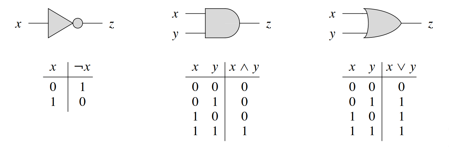
- The first NP-complete problem is the boolean satisfiability problem (or circuit satisfiability problem)
11.2 - Reduction
Cook-Levin's Theorem
- The first NP-complete problem is the boolean satisfiability problem (or circuit satisfiability problem)
\[x_0 \lor \neg x_1 \lor \neg x_3 \]
\[x_1 \lor x_2 \lor \neg x_3 \]
\[\neg x_0 \lor \neg x_2 \lor x_3 \]
\[x_0 \lor x_1 \lor x_3 \]
11.2 - Reduction
Cook-Levin's Theorem
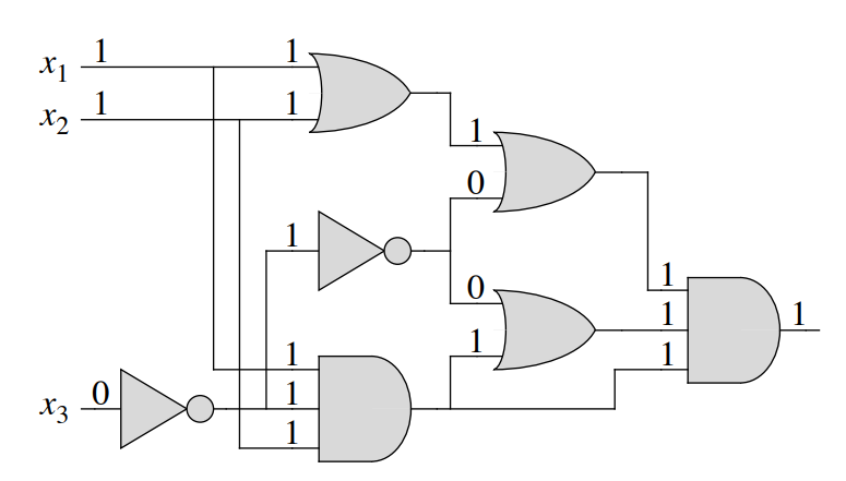
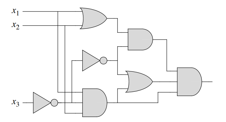
- The first NP-complete problem is the boolean satisfiability problem (or circuit satisfiability problem)
\[x_0 \lor \neg x_1 \lor \neg x_3 \]
\[x_1 \lor x_2 \lor \neg x_3 \]
\[\neg x_0 \lor \neg x_2 \lor x_3 \]
\[x_0 \lor x_1 \lor x_3 \]
\[x_0 = 1, x_1 = 1, x_2 = 1, x_3 = 1\]
1 0 0
1 1 0
0 0 1
1 1 1
11.2 - Reduction
Cook-Levin's Theorem
- The first NP-complete problem is the boolean satisfiability problem (or circuit satisfiability problem)
- The proof is beyond the scope for this unit, and it is even beyond the scope of CLRS
- SAT is what we call the mother problem, the first NP-complete problem that can be reduced to other NP-complete problems
11.2 - Reduction
NP-Complete Reduction Hierarchy
SAT
3-SAT or 3-CNF
Clique
Vertex Cover
Hamiltonian Cycle
Travelling Salesman
Subset Sum
Partition
Knapsack
11.2 - Reduction
NP-Complete Reduction Hierarchy
SAT
3-SAT or 3-CNF
Clique
Vertex Cover
Hamiltonian Cycle
Travelling Salesman
Subset Sum
Partition
Knapsack
Your
Problem
Summary
11.2 - Reduction
- Reduction must be done in polynomial-time
- A \(\le_p\) B
- if we know that A is NP-complete
- if B is in P, then we have proven P = NP
- if we don't know about B:
- if A is NP-complete, then B must be NP-hard (by definition)
- if we know that A is NP-complete
- Make sure you understand the direction of the reduction
- Are we going to do any reduction?
COMP3010 - 11.2 - Reduction
By Daniel Sutantyo


