COMP333
Algorithm Theory and Design
Daniel Sutantyo
Department of Computing
Macquarie University
Lecture slides adapted from lectures given by Igor Shparlinski and Luke Mathieson
Summary
- Algorithm complexity (running time, recursion tree)
- Algorithm correctness (induction, loop invariants)
-
Problem solving methods:
- exhaustive search
- dynamic programming
- greedy method
- divide-and-conquer
- algorithms involving strings
- probabilistic method
- algorithms involving graphs
Topics
- Probabilistic analysis
- Randomised algorithms
- Amortised analysis
Probabilistic Analysis
- Probabilistic analysis is the use of probability to analyse the running time of an algorithm
- Our main example for the discussion:
int max = 0;

for (int i = 0; i < n; i++){
    if (arr[i] > max){
        max = arr[i];
    }
}
Probabilistic Analysis
- Let us generalise the code above: we see that there are two main operations: comparison and assignment
int max = 0;

for (int i = 0; i < n; i++){
    if (arr[i] > max){
        max = arr[i];
    }
}
assign element 1 to M
for i = 2 to n:
compare element i with M
if M is less than element i:
assign i to MProbabilistic Analysis
- Suppose that comparison costs \(c_c\) and assignment cost \(c_a\)
- What is the complexity of the above algorithm?
- we have to compare all \(n\) elements for a total of \((c_c*n)\)
- do we have to do \(n\) assignments for a total cost of \((c_a*n)\)?
assign element 1 to M

for i = 2 to n:
   compare element i with M	    // cost is c_c
   if M is less than element i:
      assign i to M                 // cost is c_a
Probabilistic Analysis
- In the worst case, we have to do one assignment after each comparison, i.e. \(O(c_cn+c_an)\), but it is reasonable to expect that we don't need to do \(n\) assignments on an average input
- For the rest of our discussion, we will ignore the cost of comparison, since we have to do it anyway
- What do you think is the average-case complexity?
Probabilistic Analysis
- In order to perform a probabilistic analysis, we need to know the distribution of the input, or at least make some assumptions about it
- to do this properly, we need to understand the different types of probability distributions, which is beyond the scope of Comp333 (or even other computing units)
- However, for this example, we can assume a uniform random permutation, that is, every instance is input is equally likely
- How many different inputs are possible?
there is a total of \(n!\) possible combinations
Probabilistic Analysis
- Intuition: say there are only 4 elements
- There are 4! = 24 possible combinations
1, 2, 3, 4
1, 2, 4, 3
1, 3, 2, 4
1, 3, 4, 2
1, 4, 2, 3
1, 4, 3, 2
2, 1, 3, 4
2, 1, 4, 3
2, 3, 1, 4
2, 3, 4, 1
2, 4, 1, 3
2, 4, 3, 1
3, 1, 2, 4
3, 1, 4, 2
3, 2, 1, 4
3, 2, 4, 1
3, 4, 1, 2
3, 4, 2, 1
4, 1, 2, 3
4, 1, 3, 2
4, 2, 1, 3
4, 2, 3, 1
4, 3, 1, 2
4, 3, 2, 1
4
3
3
3
2
2
1
1
1
1
1
1
2
2
2
2
2
2
3
2
3
3
2
2
- The average is 50/24 = 2.083
Probabilistic Analysis
| n | permutation | assignments | average |
|---|---|---|---|
| 4 | 24 | 50 | 2.083 |
| 5 | 120 | 274 | 2.283 |
| 6 | 720 | 1764 | 2.450 |
| 7 | 5040 | 13,068 | 2.593 |
| 8 | 40320 | 109,584 | 2.718 |
| 9 | 362,880 | 1,026,576 | 2.829 |
| 10 | 3,628,800 | 10,628,640 | 2.929 |
| 11 | 39,916,800 | 120,543,840 | 3.020 |
| 12 | 479,001,600 | 1,486,442,880 | 3.103 |
Probability
(a little distraction)
- Probability can be counterintuitive, or at least it is easy to have the wrong intuition
- Example:
- If a family has two children, and at least one is a girl, what is the probability that both children are girls?
- If a family has two children, and the eldest is a girl, what is the probability that both children are girls?
Probability
(a little distraction)
- If a family has two children, and at least one is a girl, what is the probability that both child are girls?
- The possibilities are GG, BG, and GB, so 1/3 chance
- If a family has two children, and the eldest is a girl, what is the probability that both child are girls?
- The possibilities are GB and GG, so 1/2 chance
Probability
(a little distraction)
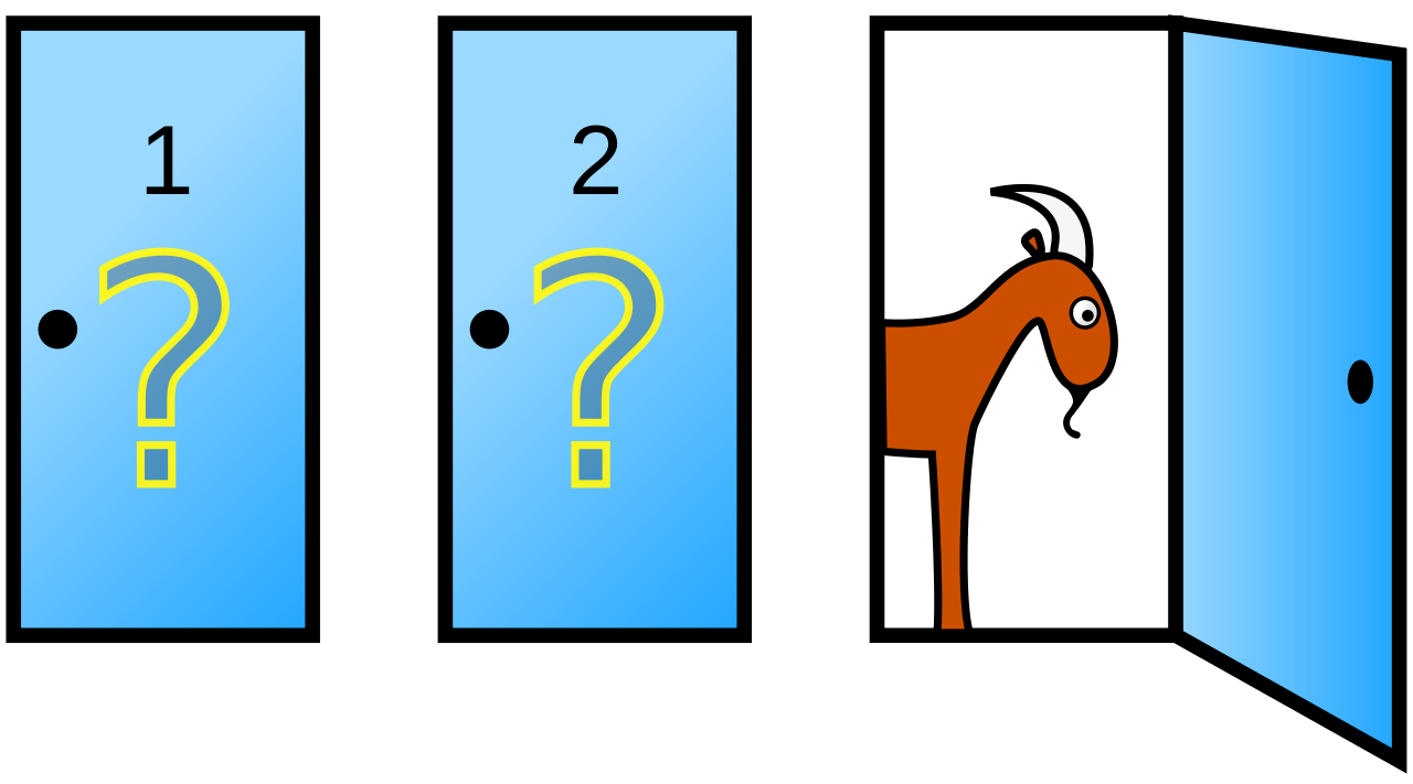
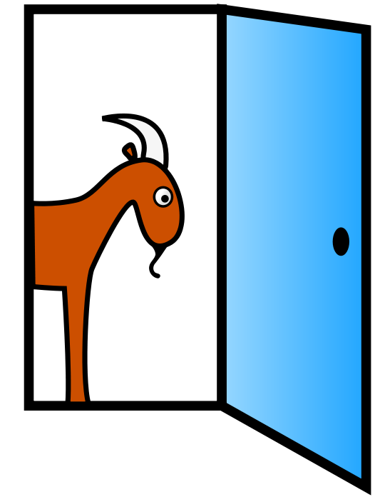
- The Monty Hall Problem:
- You are a participant in a TV game show and you are given a choice of 3 doors to open. Behind one of the doors is car, while the other doors contain nothing behind them (or maybe there is a goat)
- After you made a choice, the host opens another door (that you didn't choose) and reveals that there is a goat behind it
- Should you choose another door?
Probability
(a little distraction)
Probability
(a little distraction)
Probability
(a little distraction)
Probabilistic Analysis
| n | permutation | assignments | average |
|---|---|---|---|
| 9 | 362,880 | 1,026,576 | 2.829 |
| 10 | 3,628,800 | 10,628,640 | 2.929 |
| 11 | 39,916,800 | 120,543,840 | 3.020 |
| 12 | 479,001,600 | 1,486,442,880 | 3.103 |
- The average number of assignments you need to do doesn't seem linear
- in fact it looks logarithmic, i.e. \(O(c_a\log n)\)
Probabilistic Analysis
- The number of assignments you need to do doesn't seem linear
- in fact it looks logarithmic, i.e. \(O(c_a\log n)\)
- To derive this, you need to know about expected values
- if \(X\) is a random variable with a finite number of outcomes, say \(x_1\), \(x_2\), \(\dots\), \(x_k\) with probabilities \(p_1\), \(p_2\), \(\dots\), \(p_k\) respectively, then
\[ E[X] = \sum_{i=1}^k x_ip_i = x_1p_1 + \cdots + x_kp_k\]
Probabilistic Analysis
- For example, you are betting on the result of two coin flips:
- if the result is two heads, you double your money
- if the result is one tail and one head, you lose half your money
- if the result is two tails, you lose your money
- If you bet $\(10\), then the expected value of one game is
- \(0.25 \times 20 + 0.5 \times (-5) + 0.25 \times (-10)\) = 0
- (i.e. don't play this game)
Probabilistic Analysis
- In our example, we need to one assignment if the element we are inspecting is greater than any other element before it
- Supposing that the elements are arranged randomly, if you have \(i\) elements, each one of these elements are equally likely to be the greatest element
- So the probability of element \(i\) being the greatest element is \(1/i\)
- when you have one element, obviously that is the greatest
- when you have two elements, each has 1/2 chance of being the greatest element
- when you have three elements, each has 1/3 chance, and so on
Probabilistic Analysis
- Every time element \(i\) is the greatest element, we have to perform one assignment
- Therefore the expected number of assignment is
\[ = \sum_{i=1}^n \frac{1}{i} \]
(this is called harmonic series)
\[ \le \log n + 1\]
\[ 1 + \left(1 \times \frac{1}{2}\right) + \left(1 \times\frac{1}{3}\right) + \cdots + \left(1 \times \frac{1}{n}\right)\]
Probabilistic Analysis
- Therefore the average-case complexity of the algorithm is \(O(c_a\log n)\), which is better than the \(O(c_a n)\) worst case
- This is the standard method of estimating the average-case of an algorithm, and I am sure that you have done this before
- e.g. what is the average-case for a linear search algorithm
- All you need to do (at least in Comp333) is to find the expected number of operations
Randomised Algorithms
- The probabilistic analysis in the previous section assumes a uniform random permutation, i.e. each permutation is equally likely to occur
- Sometimes it is not possible to know the distribution of the input data, or it is not safe to make assumptions about the data
- e.g. for the previous problem we discussed (comparison and assignment), what can you do if all the inputs are always sorted ascending order?
Randomised Algorithms
assign element 1 to M

for i = 2 to n:
   compare element i with M	    // cost is c_c
   if M is less than element i:
assign i to M // cost is c_a- Given a series of values, what is the worst input for the above problem?
- What can you do?
- Sort it? It will cost \(O(c_c n \log n)\)
- Randomise it? What will this cost? Why?
Randomised Algorithms
randomise the list of elements
assign element 1 to M

for i = 2 to n:
   compare element i with M	    // cost is c_c
   if M is less than element i:
assign i to M // cost is c_a- If we randomise the input before perform the algorithm, then we will end up with an algorithm with \(O(c_a \log n)\) average-case time complexity
- Note that this is different from the probabilistic analysis we did before: even if we have no idea about the distribution of the input, we can still claim that this is the average case complexity
Probability
(a bit more distraction)
- How do you incorporate randomness into your algorithm?
- use a pseudorandom-number generator!
Probability
(a bit more distraction)
- Fisher-Yates shuffle:
- How to generate a random permutation of a finite sequence?
- Put all the numbers into a hat
- Draw them out one by one
- Complexity is \(O(n)\)
- In practice, we use a pseudorandom-number generator
- How to generate a random permutation of a finite sequence?
Randomised Algorithms
randomised algorithms vs probabilistic analysis
- Probabilistic analysis:
- we use probabilistic analysis to work out the average-case running time of a deterministic algorithm
- i.e. if you use the same input, it will always give the same output, with the exact same steps
- we use probabilistic analysis to work out the average-case running time of a deterministic algorithm
- Randomised algorithm (or probabilistic algorithm):
- a randomised algorithm incorporates some randomness in its execution, so given the same inputs, you may produce different outputs (or the same output but using different steps)
- you can derive the expected running time without knowing the distribution of the input (because you can randomise the input)
Randomised Algorithms
randomised algorithms vs probabilistic analysis
Deterministic algorithm
"Here is one input, what is the average running time?"
/\_/\
(='_' )
(, (") (")
Probabilistic algorithm
"Here is one input, what is the expected running time?"
(\____/)
( ͡ ͡° ͜ ʖ ͡ ͡°)
\╭☞ \╭☞
Randomised Algorithms
why?
- Reasons for using randomised algorithms:
- because we want to avoid input with a 'bad' distribution (as we have seen before)
- because the deterministic approach may take too long
- because you are doing cryptography or security (nonce)
- Reasons for NOT using randomised algorithms:
- because the output maybe incorrect
- because it may take too long
Randomised Algorithms
Monte Carlo and Las Vegas algorithms
- There are two major classes for randomised algorithms:
- Las Vegas algorithms
- always give correct answers, but may not finish
- Monte Carlo algorithms
- always give an answer, but may be incorrect
- Las Vegas algorithms
Randomised Algorithms
Monte Carlo and Las Vegas algorithms
Las Vegas Search Algorithm
Random rgen = new Random();
int x = 0;

while (x  != target){
  x = a[rgen.nextInt(a.length)];
}
Monte Carlo Search Algorithm
Random rgen = new Random();
int x = 0;

while (x  != target && count < max){
  count++;
  x = a[rgen.nextInt(a.length)];
}
Randomised Algorithms
Monte Carlo and Las Vegas algorithms
- You can convert a Las Vegas algorithm into a Monte Carlo algorithm:
- put a limit on the number of operations before giving up and then returning something
- You can convert a Monte Carlo algorithm into a Las Vegas algorithm:
- do not return an answer unless you are certain that it is correct
Randomised Algorithms
(minor) examples
- Bogosort
also known as permutation sort, stupid sort, slowsort,
&#%@sort, shotgun sort, and monkey sort
- Quicksort
Randomised Algorithms
Quicksort
Randomised Algorithms
Quicksort
- The worst-case running time for quicksort happens when at each partition, you create one subproblem with \(n-1\) elements, and another subproblem with 0 elements
- \(T(n) = T(n-1) + T(0) + \Theta(n) = \Theta(n^2)\)
- The best-case is when you have an even split, two subproblems of size around \(n/2\)
- \(T(n) = 2T(n/2) + \Theta(n) = \Theta(n\log n)\)
Randomised Algorithms
Quicksort
- Note that in reality, when performing a quicksort, on average you will get 'good splits' and 'bad splits', but you would have to be extremely unlucky to get a series of 'bad' splits (assuming you always take the first element as the pivot)
- Even in the case of 'bad' splits, the complexity is not so bad:
- \(T(n) = T(9n/10) + T(n/10) + \Theta(n)\) = ???
(we will cover this in the workshop)
Randomised Algorithms
Randomised Quicksort
- In the randomised version of quicksort, we do not use the first element of the array as the pivot
- Instead we pick a random element in the array as the pivot, thus removing the possibility of having to work with a series of degenerate inputs
- The proof is in Section 7.4 of CLRS (pg. 182-183), but it is not examinable
Randomised Algorithms
Randomised Quicksort
- Is randomised quicksort a Las Vegas or a Monte Carlo algorithm?
- How do you convert it into a Monte Carlo algorithm?
Randomised Algorithms
Matrix Multiplication Verification
-
Problem: given three \(n \times n\) matrix, \(A\), \(B\), and \(C\), verify whether or not \(AB = C\)
- The naive method for solving this is \(O(n^3)\) (i.e. do the matrix multiplication)
- this can actually be done faster using Strassen Algorithm
\[\begin{bmatrix} 5 & 5 & 3 \\ 7 & 1 & 3 \\ 4 & 1 & 5 \end{bmatrix}\]
\[\begin{bmatrix} 9 & 3 & 2 \\ 4 & 2 & 1 \\ 7 & 7 & 7 \end{bmatrix}\]
\[\begin{bmatrix} 86 & 46 & 36 \\ 88 & 44 & 36 \\ 75 & 49 & 44\end{bmatrix}\]
?=?
Randomised Algorithms
Matrix Multiplication Verification
- A probabilistic approach:
- Choose a random vector \(x\), then multiply both sides by \(x\)
\[\begin{bmatrix} 5 & 5 & 3 \\ 7 & 1 & 3 \\ 4 & 1 & 5 \end{bmatrix}\]
\[\begin{bmatrix} 1 \\ 1 \\ 1 \end{bmatrix}\]
\[\begin{bmatrix} 86 & 46 & 36 \\ 88 & 44 & 36 \\ 75 & 49 & 44\end{bmatrix}\]
\[\begin{bmatrix} 9 & 3 & 2 \\ 4 & 2 & 1 \\ 7 & 7 & 7 \end{bmatrix}\]
\[\begin{bmatrix} 1 \\ 1 \\ 1 \end{bmatrix}\]
\[\begin{bmatrix} 168 \\ 168 \\ 168 \end{bmatrix}\]
\[\begin{bmatrix} 168 \\ 168 \\ 168 \end{bmatrix}\]
=
=
Randomised Algorithms
Matrix Multiplication Verification
\[\begin{bmatrix} 5 & 5 & 3 \\ 7 & 1 & 3 \\ 4 & 1 & 5 \end{bmatrix}\]
\[\begin{bmatrix} 1 \\ 1 \\ 1 \end{bmatrix}\]
\[\begin{bmatrix} 86 & 46 & 36 \\ 88 & 44 & 36 \\ 75 & 49 & 44\end{bmatrix}\]
\[\begin{bmatrix} 9 & 3 & 2 \\ 4 & 2 & 1 \\ 7 & 7 & 7 \end{bmatrix}\]
\[\begin{bmatrix} 1 \\ 1 \\ 1 \end{bmatrix}\]
\[\begin{bmatrix} 168 \\ 168 \\ 168 \end{bmatrix}\]
\[\begin{bmatrix} 168 \\ 168 \\ 168 \end{bmatrix}\]
=
=
can be done in \(O(n^2)\)
sure!
\[\begin{bmatrix} 14 \\ 7 \\ 21 \end{bmatrix}\]
\[\begin{bmatrix} 5 & 5 & 3 \\ 7 & 1 & 3 \\ 4 & 1 & 5 \end{bmatrix}\]
\[\begin{bmatrix} 168 \\ 168 \\ 168 \end{bmatrix}\]
=
can this be done in \(O(n^2)\)?
Randomised Algorithms
Matrix Multiplication Verification
- If \(AB \ne C\), then for a randomly chosen vector \(x\), the probability that \(ABx = Cx\) is small
- Even if it is not small, we can use a technique known as probability amplification:
- Let's suppose that there 50% chance that if \(AB \ne C\), we have \(ABx = Cx\)
- If you pick another random vector \(x_1\) and \(x_2\), what are the chances that \(ABx_1 = Cx_1\) and \(ABx_2 = Cx_2\)?
Randomised Algorithms
Matrix Multiplication Verification
- Algorithm:
- Pick a random vector \(x\)
- Compare \(ABx\) to \(Cx\)
- If you perform this 10 times and each time \(ABx = Cx\), the probability of this happening is \(0.5^{10}\) = 0.0009765625
- As soon as it is false, i.e. as soon as \(ABx \ne Cx\), then you know that \(AB \ne C\)
- The cost of this approach is still \(O(n^2)\)
Randomised Algorithms
Matrix Multiplication Verification
- Is the matrix multiplication verification algorithm a Monte Carlo algorithm or a Las Vegas algorithm?
Randomised Algorithms
Summary
- To determine the average-case complexity of a deterministic algorithm, we use probabilistic analysis
- Randomised algorithm:
- introduce some randomisation in the algorithm
- can handle degenerate input cases (by randomising the input)
- can be fast, be gives incorrect answer (Monte Carlo)
- may 'never' finish (Las Vegas)
Primality Testing
- Problem: given an integer \(n\), determine whether or not it is a prime number
- Primality testing is a very important algorithm in cryptography
- The topic has been studied extensively and there are numerous algorithms that you can use for primality testing
- most of them require heavy mathematics (elliptic curves, cyclotomic fields, number fields), so we won't be discussing them in Comp333
- however some of the algorithms are quite easy to understand, and more importantly, they are probabilistic!
Primality Testing
simple methods
- The simplest method of primality testing is to simply try every integer value less than \(\sqrt{n}\)
- complexity is \(O(\sqrt{n})\) divisions
- is this polynomial?
| 10,000 | 100 |
| 20,000 | 141 |
| 30,000 | 173 |
| 40,000 | 200 |
| 50,000 | 223 |
\(n\)
\(\sqrt{n}\)
| 14 |
| 15 |
| 15 |
| 16 |
| 16 |
input size
Primality Testing
simple methods
- The simplest method of primality testing is to simply try every integer value less than \(\sqrt{n}\)
- complexity is \(O(\sqrt{n})\) divisions
- this is exponential in complexity!
| 14 | 16383 | 127 |
| 15 | 32767 | 181 |
| 16 | 65535 | 255 |
| 17 | 131017 | 362 |
| 18 | 262143 | 511 |
input size
\(\sqrt{n}\)
\(n\)
Primality Testing
simple methods
- The simple method is very slow, but it is the basis for the more advanced methods (can be improved using sieve of Erastosthenes)
Primality Testing
simple methods
- Nevertheless, using the simple method is simply not fast enough because it is exponential to the size of the input
- It has been proven that you can perform primality testing in \(O((\log n)^{12})\) (this is polynomial time to the number of bits)
- this was the famous AKS primality test, and was improved further later on
- in practice, it is a galactic algorithm, i.e. an algorithm which runs faster than any other algorithm for probably that are sufficiently large, where 'sufficiently large' here means 'galactically large'
Primality Testing
Fermat's primality test
\[a^{p-1} \equiv 1 \pmod p\]
- Fermat's Little Theorem:
- if \(p\) is prime, then for all integer \(a\) such that \(\gcd(a,p) =1\), we have
- if \(p\) is prime, then for all integer \(a\) such that \(\gcd(a,p) =1\), we have
Primality Testing
Fermat's primality test
\[a^{p-1} \equiv 1 \pmod p\]
- for \(1 \le x < p\), we have
\[ax \equiv bx \mod p\]
if and only if \(a = b\)
- in other words:
- Proof of Fermat's little theorem:
\(a, 2a, 3a, 4a, \dots, (p-1)a\) are all distinct
\(a\times 2a\times \dots \times(p-1)a = 1\times2\times3 \times \dots\times(p-1) \pmod p\)
- so:
\(a^{p-1} = 1\pmod p\)
Primality Testing
Fermat's primality test
- Using Fermat's little theorem for primality testing is simple:
- Input: an integer \(n\)
- Output: returns true if \(n\) is a probable prime, false otherwise
-
Algorithm:
- pick a base \(a\)
- perform fast exponentiation to compute \(a^{n-1}\)
- if \(a^{n-1} \not\equiv 1 \pmod n\), return false
- otherwise return probable prime
Primality Testing
Fermat's primality test
- Why probable prime?
- Unfortunately for a non-prime \(n\), there is a chance that \(n\) also satisfies the equation
\[a^{n-1} \equiv 1 \pmod n\]
- if \(n\) is non-prime, then we call such integer \(a\) a false witness
- example: \(3^{90} \equiv 1 \pmod {91} \), \(4^{90} \equiv 1 \pmod {91}\)
- but \(5^{90} \equiv 64 \pmod{91}\)
- for 91, there are quite a false witnesses: 1, 3, 4, 9, 10, 12, 16, 17, 22, 23, 25, 27, 29, 30, 36, 38, 40, 43, 48, 51, 53, 55, 61, 62, 64, 66, 68, 69, 74, 75, 79, 81, 82, 87, 88, 90
Primality Testing
Fermat's primality test
- There is also a special type of integers called Carmichael numbers, e.g. \(561 = 3 \times 11 \times 17\)
- every integer \(x\) coprime to a Carmichael number \(n\) satisfies \(x^{n-1} \equiv 1 \pmod n\), i.e. it is a false witness
- Nevertheless, we can still use Fermat's primality testing using multiple bases to sniff out these false witnesses (probability amplification), although the chances aren't that great if you hit a Carmichael number
- So Fermat's primality test is a Monte Carlo algorithm
\[a^{n-1} \equiv 1 \pmod n\]
- We can improve Fermat's primality testing further using the Miller-Rabin test. Here is an example to illustrate the algorithm:
- we want to test if 561 is prime (it is a Carmichael number)
- we have \(560 = 2^{4} \times 35\)
- pick a random base, say \(a = 100\) (note \(\gcd(561,100) = 1\))
- \(100^{35} \pmod {561} = 298\)
- \(100^{70} \pmod {561} = 166\)
- \(100^{140} \pmod {561} = 67\)
- \(100^{280} \pmod {561} = 1\)
- \(100^{560} \pmod {561} = 1\) we say that 561 is composite
- we want to test if 561 is prime (it is a Carmichael number)
Primality Testing
Miller-Rabin test
\[a^{n-1} \equiv 1 \pmod n\]
- Let us see what happens if we test an actual prime:
- \(569 = 8 \times 71 + 1\)
- \(568 = 2^3 \times 71\)
- pick a random base, \(a = 100\)
- \(100^{71} = -1 \pmod{569}\)
- \(100^{142} = 1 \pmod{569}\)
- \(100^{284} = 1 \pmod{569}\)
- \(100^{568} = 1 \pmod{569}\), we conclude \(569\) is a probable prime
Primality Testing
Miller-Rabin test
- To understand the explanation, we need one little fact:
- for a prime \(p\), the equation \(x^2 \equiv 1 \pmod p\) only has two solutions: -1 and 1
- quick proof: if \(a^2 \equiv 1 \pmod p\), this means
- \(a^2 - 1 \equiv 0 \pmod p \quad\rightarrow\quad (a+1)(a-1) \equiv 0 \pmod p\)
- so the only possible solutions are 1 or -1
- quick proof: if \(a^2 \equiv 1 \pmod p\), this means
- for a prime \(p\), the equation \(x^2 \equiv 1 \pmod p\) only has two solutions: -1 and 1
Primality Testing
Miller-Rabin test
- Fact: for a prime \(p\), the equation \(x^2 \equiv 1 \pmod p\) only has two solutions: -1 and 1
- Suppose \(a^{n-1} \equiv 1 \pmod n\)
- take the square root of \(a^{n}\): if \(n\) is indeed prime, then you will either get -1 or 1
- the square root of \(a^{n-1}\) is \(a^{(n-1)/2}\)
- so if \(a^{(n-1)/2}\) is not 1 or -1, then we know \(n\) is not a prime
- if \(a^{(n-1)/2}\) is 1 or -1, then take its square root again
- the square root of \(a^{(n-1)/2}\) is \(a^{(n-1)/4}\)
- and so on
Primality Testing
Miller-Rabin test
Primality Testing
Miller-Rabin test
- In practice, the implementation of Miller-Rabin test is as follows:
- given \(n\), find \(s\) such that \((n-1) = 2^sq\) for some odd \(q\)
- with \(n = 569\), we start with \(a^{71}\)
- \((a^{71})^2 = a^{142}\), \((a^{142})^2 = a^{284}\), \((a^{284})^2 = a^{568}\)
- with \(n = 569\), we start with \(a^{71}\)
- pick a random \(a \pmod n\)
- if \(a^q = 1\), then we say that \(n\) is a probable prime
- if not, then compute \(a^{2^iq}\), \(i = 0, 1, \dots, (s-1)\) to see if it equals -1
- if it does, then we say it is a probable prime
- if it never hits -1, then we say that the number is composite (why?)
- given \(n\), find \(s\) such that \((n-1) = 2^sq\) for some odd \(q\)
Primality Testing
Miller-Rabin test
- If the algorithm states that \(n\) is composite, then we know this is correct
- If the algorithm states that \(n\) is a probable prime, it has at most \(1/4\) chance of being incorrect (on average, it is less)
COMP333 Algorithm Theory and Design - W8 2019 - Probabilistic Algorithms
By Daniel Sutantyo
COMP333 Algorithm Theory and Design - W8 2019 - Probabilistic Algorithms
Lecture notes for Week 8 of COMP333, 2019, Macquarie University


