Applied Microeconomics
Lecture 6
BE 300
Plan for Today
Costs and output decisions
Profit maximization
Cost of Cows Case
Costs and Output Decisions
Thinking Like an Economist: understand which costs matter for which decisions.
Costs that are important from an economic (and managerial) perspective are not always identical to those that are measured by accountants (see this today in the case)
- Some measured costs are irrelevant for decision-making, e.g., sunk costs
- Some costs that are not measured are important, e.g., opportunity costs
Costs and Revenue
Profit is total revenue minus total cost.
To maximize profit (short run), firms need to think
about two important decisions:
Decision 1: How much should I produce?
Decision 2: Should I shut down (if I'm making a loss)?
Costs: Output Decisions
When deciding how much to produce, firms think about how much additional output will cost to produce and weight that with how much revenue the additional output will bring in.
Cost of one more unit = marginal cost.
Revenue brought in for one more unit=marginal revenue.
Marginal Revenue
Marginal revenue is exactly analogous to marginal cost:
- The change in total revenue from selling one more unit of a product (MR = ΔTR/ΔQ, when ΔQ = 1), or
- the derivative (MR = dTR/dQ)
The incremental revenue from selling one more unit.
Marginal Revenue
Recall TR is equal to P*Q and assume you face a linear, downward sloping demand curve.
If price is fixed, increasing Q raises TR.
If quantity is fixed, increasing P raises TR.
But what if both are varying?
To sell more, the you must lower the price--inherent tension between expanding production but not wanting to lower the price too much.
Marginal Revenue
Remember from our discussion of elasticity: As you move along the demand curve, total revenue first increases then decreases.
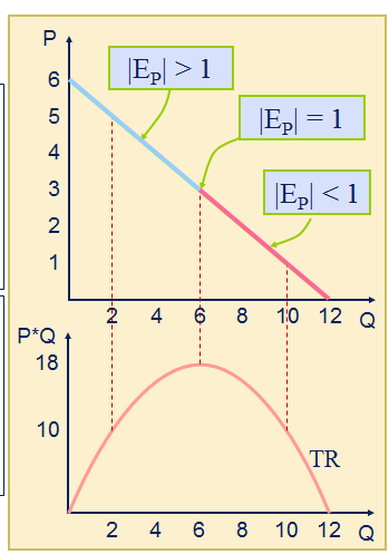
Marginal Revenue
We can graph the change in revenue like we graph total revenue.
In the elastic region of demand, marginal revenue is (positive or negative)?
In the inelastic region of the demand curve, marginal revenue is (positive or negative)?
Marginal Revenue
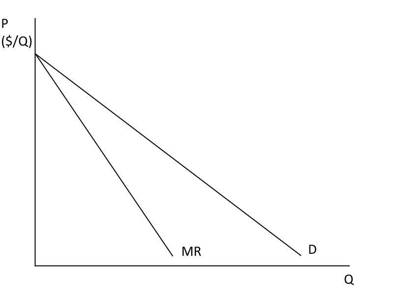
When you face a downward sloping linear demand curve, we can write total revenue is:
TR=(P*Q).
P = a – bQ
So TR = (a – bQ)Q = aQ – bQ^2
MR = a - 2bQ
In the linear case, MR has the same intercept but twice the slope as the demand curve.
Marginal Revenue
MR=0 when the elasticity of demand = ?
Profit Maximizing
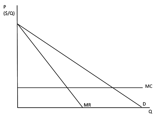
Say you have a flat cost per unit.
Profit Maximizing
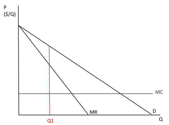
You're currently producing Q1. What is the price you're charging?
Profit Maximizing
You are thinking about increase Q by one unit. How much will it cost you to produce this unit? How much revenue will this unit bring in?
Profit Maximizing
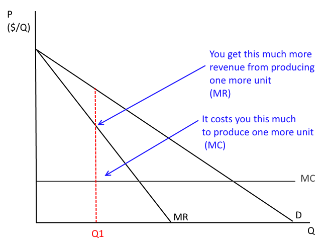
So, good idea to produce one more unit?
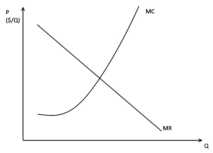
Profit Maximizing
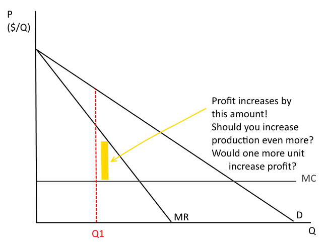
Profit Maximizing
If the marginal revenue is above the marginal cost, increasing Q will increasing profit!
Profit Maximizing
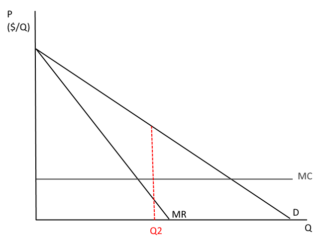
Now we're producing at Q2. What was the cost to produce this unit? How much did it increase our revenue?
Profit Maximizing
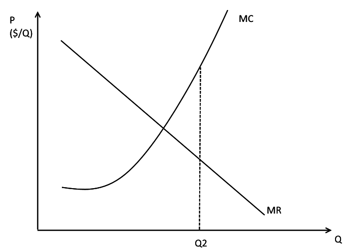
Same logic with an increasing MC curve--you don't want to produce units if MC > MR
Profit Maximization
For example
(Don't pay much attention to what they call "fixed" or "variable" pricing)
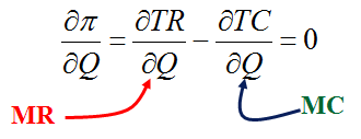
Profit Maximizing
So... where is profit maximized?
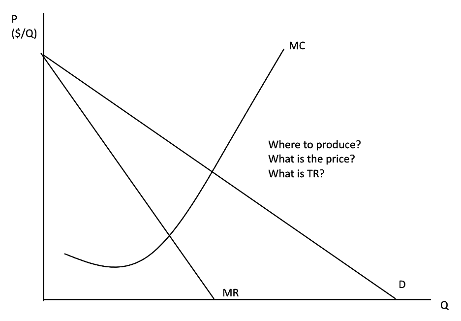
Profit is maximized when MC=MR
Profit Maximization
Profit is maximized when MR=MC (just like consumer surplus is maximized when the marginal benefit of consumption equals the marginal cost (price) of consumption).
You can also see this using calculus:
Profit=TR-TC.
Take first derivative wrt q and set equal to 0:
Profit Maximization
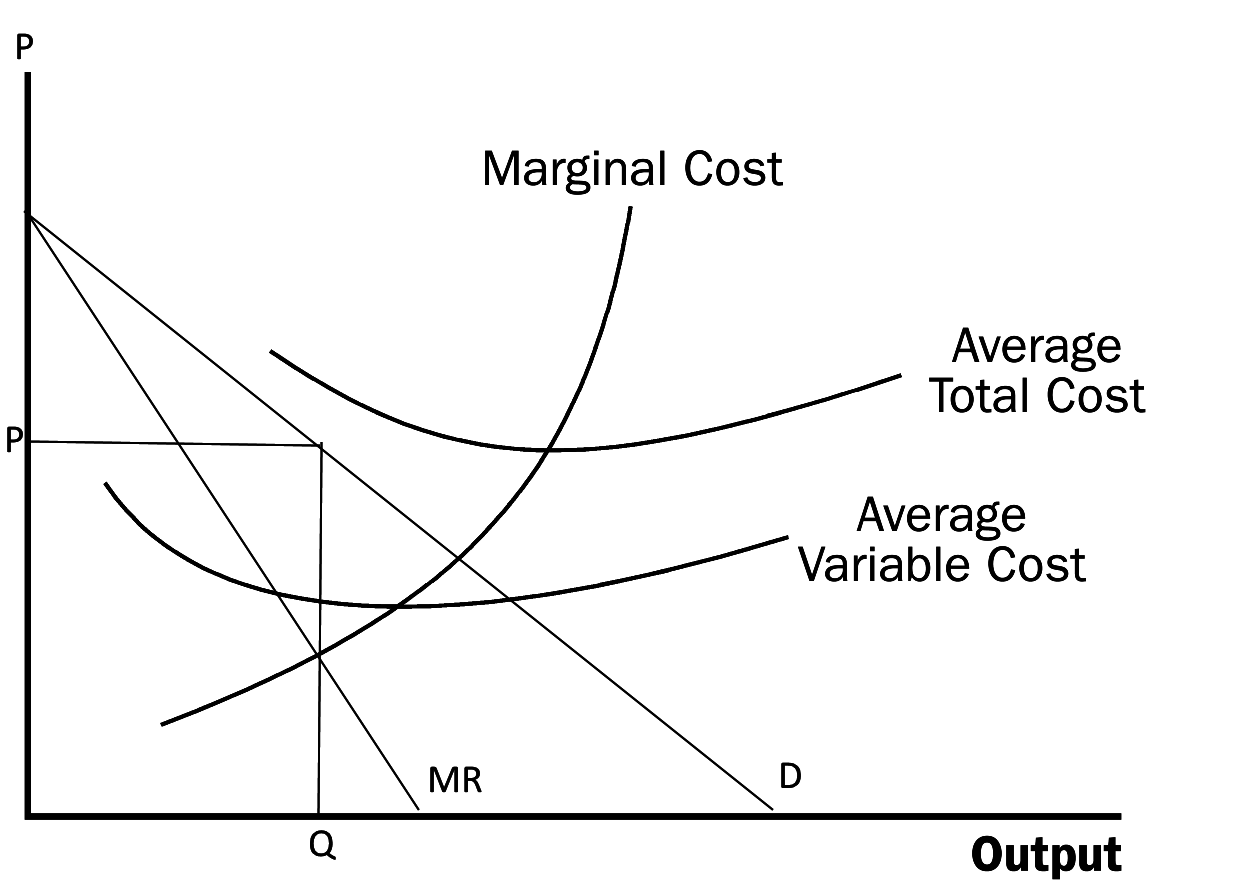
Profit Maximization
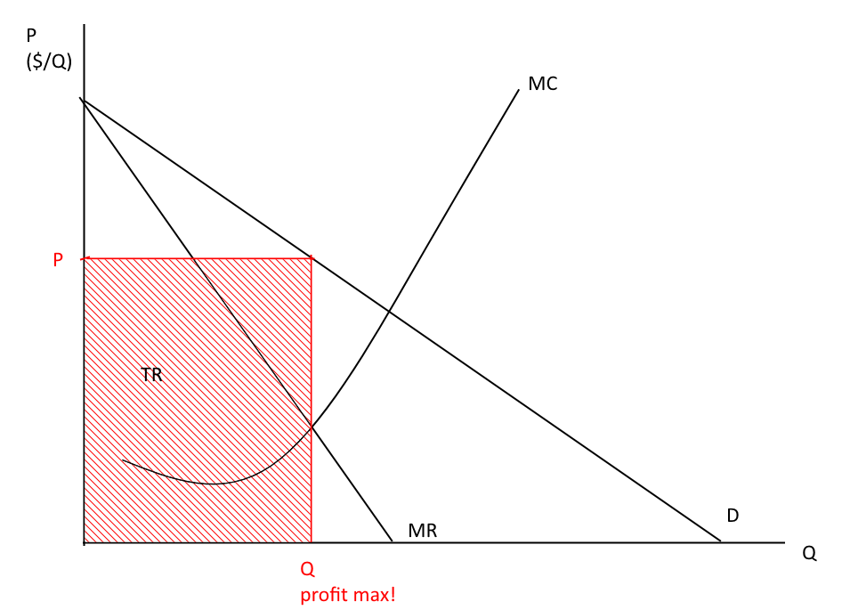
Remember to read price off of the demand curve (not MR curve!)
Profit Maximization
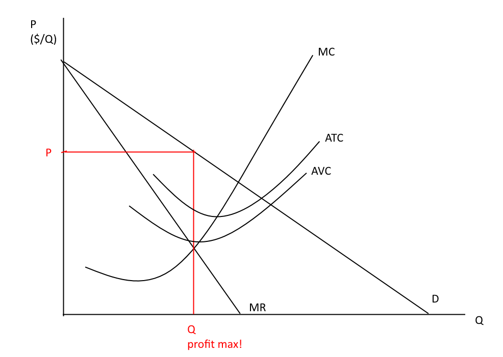
Let's make things a bit more complicated...
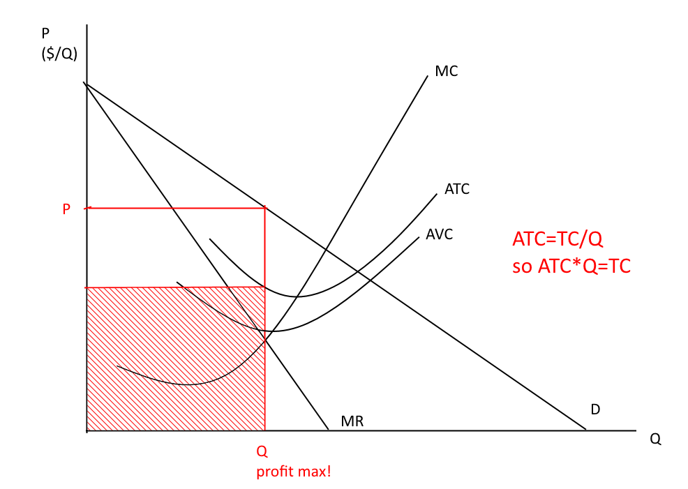
ATC=(___)/Q
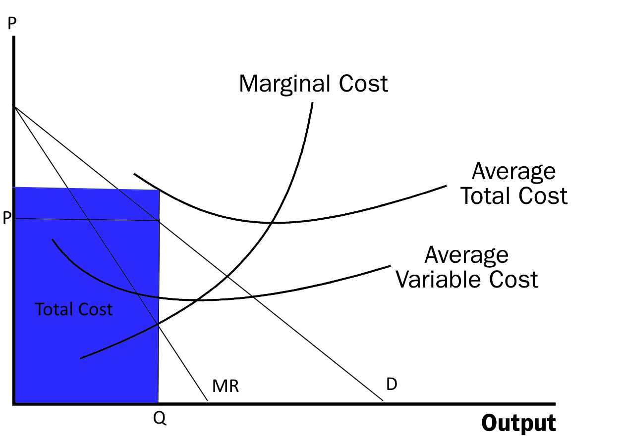
Profit Maximization
Where is total cost at the profit max Q on the figure?
Profit Maximization
Profit Maximization
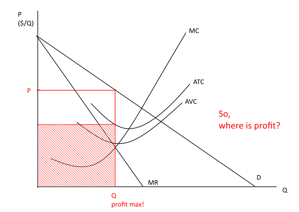
Profit Maximization
Profit Maximization
What about this scenario? Is the firm earning a profit?
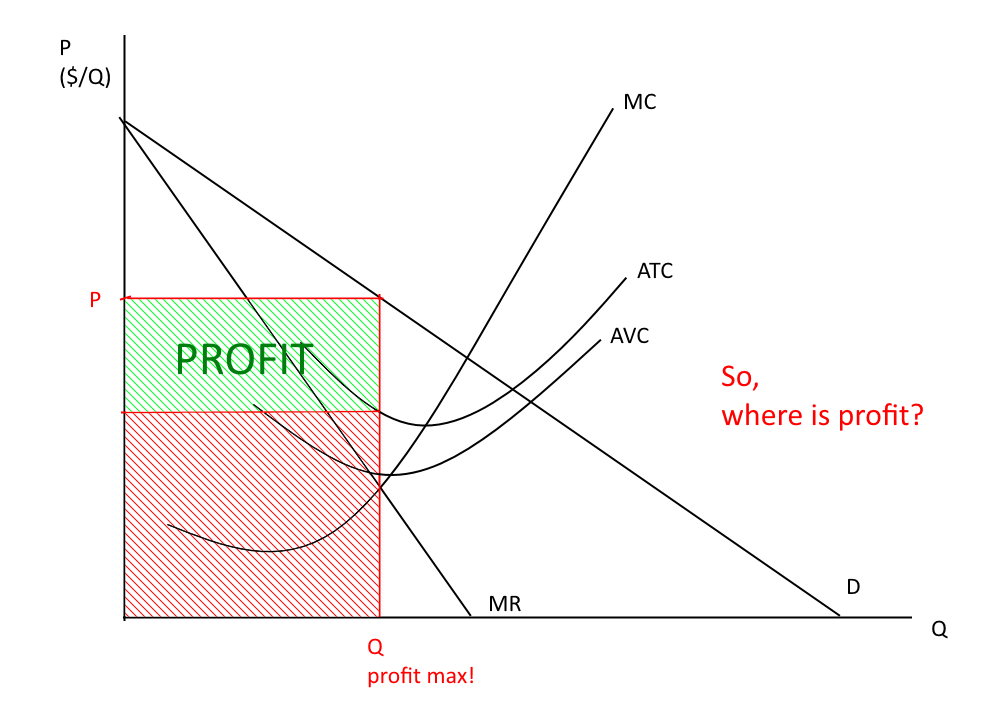
Profit Maximization
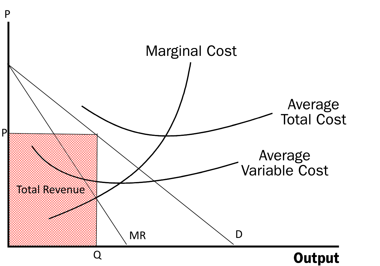
Total revenue
Profit Maximization
Profit Maximization
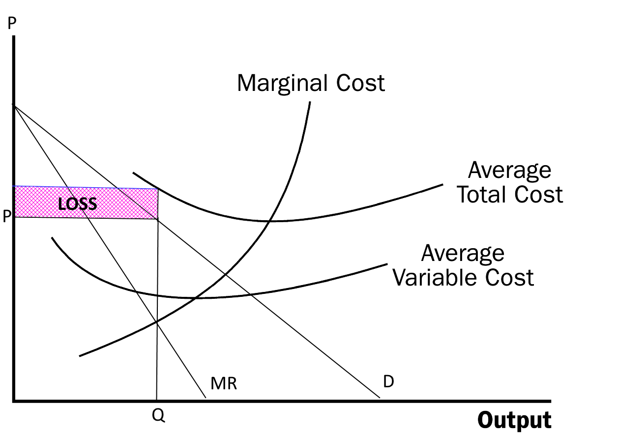
So, should the firm shut down?
Profit Maximization
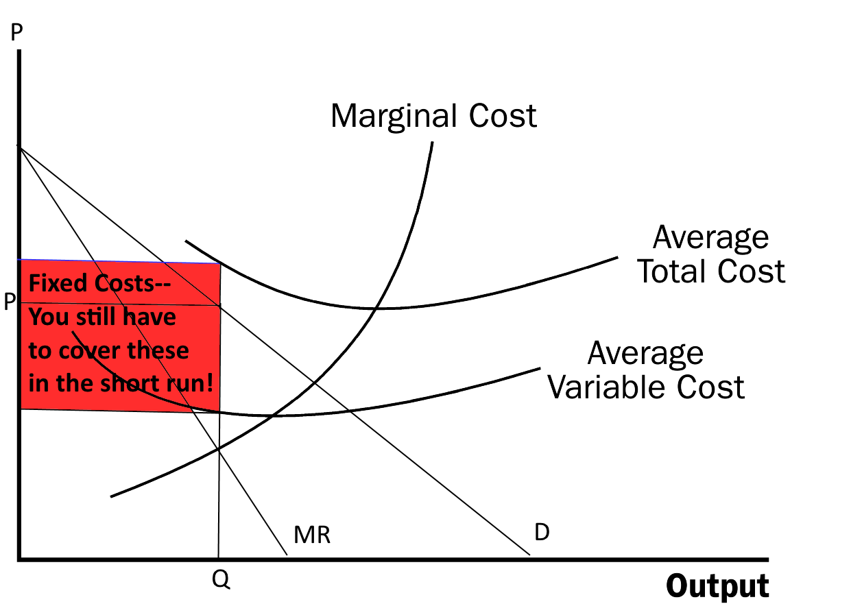
As long as price is above AVC, you are able to cover your operational expenses and some of your fixed costs.
Profit Maximization
As long as price is above AVC, you are able to cover your operational expenses and some of your fixed costs even though you are losing money.
Shut down only if P < AVC.
Moo'ved on Out?
Don’t Look of Gift Cow in the Mouth?
Nearly half of rural households in India own cow or buffalo
- Milk, dung, calf
- State/federal policies reinforce the hypothesis that livestock investments produce more value than cash
If a farmer doesn’t have to put up the money to buy a cow/buffalo he or she receives the operating profits from the milk, dung, and calves…..BUT…
Cow Costs
Cow Case
Cow Markets are Important but Inefficient
Poor rural households often use livestock assets for output and to smooth consumption.
- Dairy animals are the most common asset purchased with microfinance loans in rural areas
Market for cows has large degree of asymmetric info (about quality) – generates inefficiency in trading
- Impossible to tell quality unless cow is milking (i.e, not dry)
Does owning cows and buffalo really pay off?
CASE: Should HHs own cow or buffalo?
Given:
- The policy emphasis on “in-kind” transfers of livestock, and
- The inefficient market for their trading/sale
We need to know whether cows and buffalo really are profitable investments (or gifts)
Ladies and gentlemen, turn on your cow-culators
Cowculations
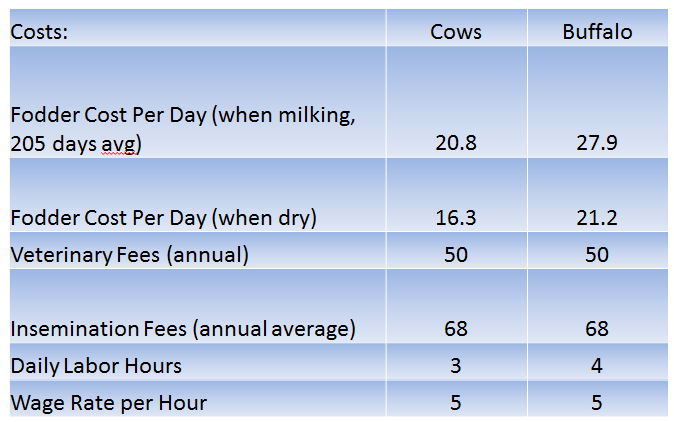
Of the costs listed in Table 1, categorize each as fixed or variable. Assume the farmer already owns a cow or buffalo, but can choose whether to produce milk or not.
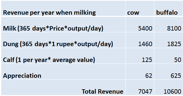
TR over 3 outputs: Milk, Dung and Calves + appreciation
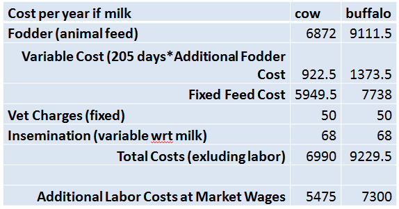
Costs
Now let's look at the costs...
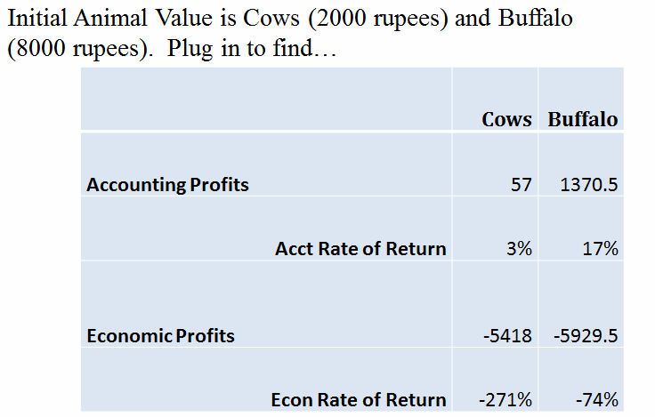
Are Cows Profitable?
"Accounting" profit (doesn't take into account opportunity cost):
For a cow: 7047-6990=57 rupees
For a buffalo: 10600-9229.5=1370.5 rupees
Economic profit (taking into account opportunity cost of labor):
For a cow: 7047-6990-5475=-5418
For a buffalo:10600-9229.5-7300=-5929.5
Rate of Return
Milk and Calves
Let's assume the farmer won't just let the cow die!
How much more do you have to pay in terms of costs to produce milk?
Additional cost of producing milk=extra feed + insemination fee=(922.5+68)=$990.5
Additional benefit of producing milk and calves=5400+125=5525
Cow Case
Re-compute economic profits when children provide all the labor? Why might there be a preference for child labor in livestock husbandry?
Children earn lower wages--they have a lower opportunity cost of caring for animals.
Cow Case
What are children's average wages outside the home?
How will this change economic profits?
Cow Case
Assume the market for milk in rural India is perfectly competitive and consumer demand in Uttar Pradesh is given by 𝑃_𝑚𝑖𝑙𝑘=40−1.6×𝑄_𝑚𝑖𝑙𝑘 (where Q is measured in millions of liters of milk).
Compute the price of milk at which the typical household would just break even, i.e. have zero economic profits, for both cows and buffalo.
- Would there be demand for milk at that price?
- If so, how much total demand would there be?
Cow Case
Profits = MilkRev(Pm*Qm) + DungRev(Pd*Qd) + CalfRev (Pc*Qc)+Appreciation
– Total Econ Cost
Set profits to zero and solve for Breakeven Price Pm
Pm=(Total Cost - Dung Revenue - Calf Rev - Appreciation)/Q_m
Breakeven Price:
Cows: Pm=(6990+5475-1460-125-62)/481.8=22.44 rupees
Buffalo: Pm=(9229.5+7300-1825-50-625)/693.5=20.23 rupees
At both prices there is positive consumption (plug in to demand function)
Cow Case
Now assume that there are only cows and the price of milk is 11.2. What is your estimate for the number of cows in Uttar Pradesh in 2007? If there are no changes in technology or production efficiency, what do you predict should happen to the number of cows over the long run? Explain your answer.
Cow Case
Assume instead that cow milk and buffalo milk are perfect substitutes and households are profit maximizers. In the long run, should we observe more cows or more buffalo? Why?
Cow Case
Compute a lower bound on the implied religious or social value of the average cow and the average buffalo when labor costs are included in total costs of the average animal. Why is this a “lower bound” estimate?
Cow Case
Critics of this religion-based explanation have noted that buffalo, unlike cows, have no religious value, and yet even these animals seem to exhibit negative returns. What are some other reasons for the continued existence of cows and buffalo?
In Conclusion...
From Short-Run to Long-Run Costs
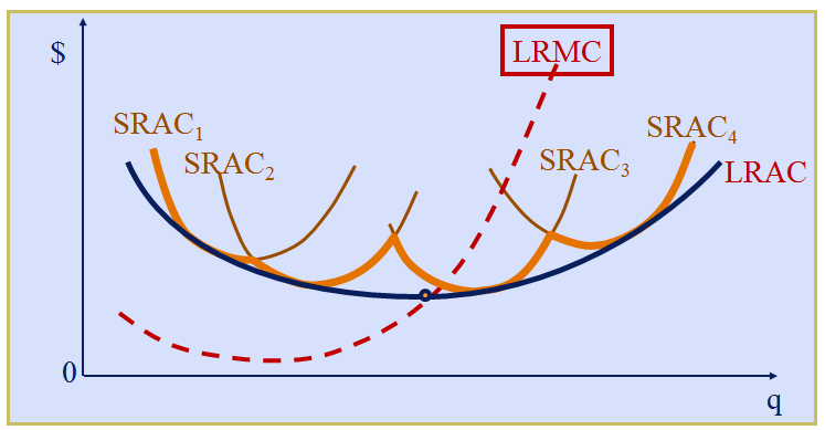
LRAC is the “envelope” of the SRAC curves & is typically flatter than any SRAC (This shows the increased flexibility – we can change the size of the plant (store, facility) now so there is no crowding)
Long Run Average Total Costs
Long Run Average Cost
Economies of Scale means that output can be doubled for less than a doubling of cost (i.e., LRAC is decreasing).
What are the sources of economies of scale?
Long Run Average Cost
Possible sources of Economies of Scale:
- Specialization of workers & machinery => greater efficiency & lower costs per unit
- Scale can provide flexibility => greater efficiency
- May be able to purchase inputs at lower cost b/c buying in larger quantities (or can allow suppliers to achieve economies of scale)
Long Run Average Cost
Diseconomies of Scale means that costs more than double when output is doubled (i.e., LRAC is increasing for some q).
What might cause diseconomies of scale?
Long Run Average Cost
Possible reasons for diseconomies of scale:
Complexities of managing a larger firm => greater inefficiency
Availability of key supplies may be limited, and additional demand may require finding more expensive sources for those supplies, pushing up their cost
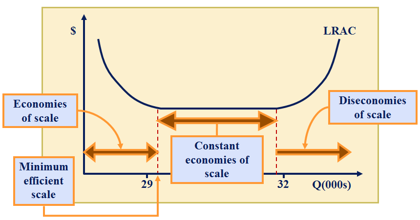
Minimum Efficient Scale (MES)
Definition: The minimum size of a firm or plant that allows it to achieve all available economies of scale
Mathematically: smallest output level at which LRAC is minimized
What do average cost curves really look like?
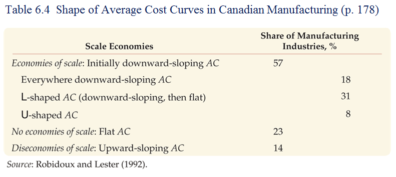
We often can’t estimate what we don’t observe – some L-shaped AC curves likely slope up at some output level, but we don’t observe firms operating in that region.
Liquid Costs: Costs of Beer and Oil

BEER: constant returns to scale in the long-run (can always add more tanks or bottling machines.) But stuck with existing capital in short run. (Perloff and Branders 2014)
Liquid Costs: Costs of Beer and Oil

OIL: Long run decreasing returns to scale if can build larger diameter pipes.
Changes to Long Run Costs
Three main factors shift long-run cost curves:
- Economies of scope
- Learning economies
- Input prices and technological change
Economies of Scope
Fundamental strategic question: should a firm focus on a single product or offer many different products? Answer partly depends on how production and costs interact!
Economies of Scope
Economies of scope are positive if:
The cost of joint production of two (or more) distinct products is
less than the cost of producing the same amount of each product
separately
i.e. C(q1,q2) < C1(q1, 0) + C2(0, q2)
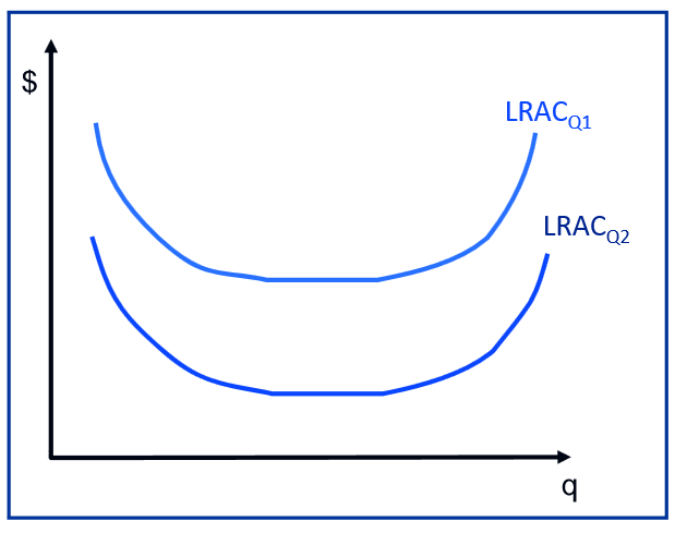
With economies of scope, the whole LRAC function for q1 shifts down as production of q2 increases (and vice versa)
Economies of Scope
Some production processes naturally exhibit economies of scope:
-
B-Schools: BBA, MBA, PhD, EMBA
-
Lamb meat and wool; beef and leather
-
McDonald's: breakfast and lunch
-
Amazon: product sales & cloud computing
Any others?
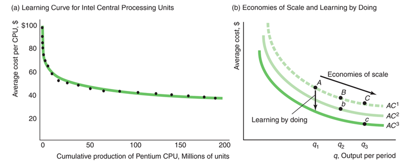
Learning Economies
Learning Curve vs. Economies of Scale
Learning by doing for Intel (see text p. 182)
Technological Change
Permanent changes in the price of key inputs will shift long-term cost curves up or down.
-
Example: microprocessors in the computer industry
Technological change makes new combinations of inputs possible, leading to lower production costs.
Example: better logistics lead to more efficient equipment use in the trucking industry.
Regulatory change can affect production costs.
Example: emission standards and pollution permitsCost Fundamentals: Key Topics
- An opportunity cost is the implicit cost associated with using a resource in a particular endeavor
- A sunk cost is an expenditure that once made cannot be recovered
- Total economic cost includes opportunity costs and disregards sunk costs
- Average cost is total economic cost divided by output
- Marginal cost is the change in total economic cost to produce one more unit of output
Cost Fundamentals: Key Topics
The short run is the period within which firms cannot modify the size of their facilities. Because of this, some costs are fixed in the short run.
The “Law of Diminishing Returns” says that in the short run, average costs (variable and total) must at some point increase
Cost Fundamentals: Key Topics
The long-run ATC curve is just the envelope of the short-run ATC curves
We care about the long run average cost curve because it tells us efficient plant sizes
Economies of scale exist when one gets more than an x% increase in output from increasing all inputs (labor, materials, capital and equipment) by x%
Next Time:
TUESDAY Feb. 3
Textbook: Ch. 2 intro, 2.3 – 2.4, 2.6; Ch. 7.5; Ch. 8 intro, 8.1–8.3.
THURSDAY Feb. 5
Textbook: Ch. 2.5; pp. 265 – 268; Ch. 9 intro, 9.1 – 9.4; Ch. 8.4; Ch. 16 intro & Ch. 16.1
Lecture 6
By umich


