Applied Microeconomics
Lecture 7
BE 300
Plan for Today
Long Run Costs
Competitive Markets
From Short-Run to Long-Run Costs
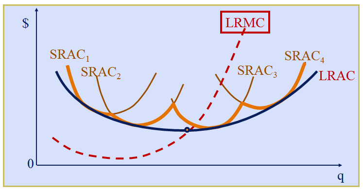
LRAC is the “envelope” of the SRAC curves & is typically flatter than any SRAC (This shows the increased flexibility – we can change the size of the plant (store, facility) now so there is no crowding
Long Run Average Total Costs
Long Run Average Cost
Economies of Scale means that output can be doubled for less than a doubling of cost (i.e., LRAC is decreasing).
Long Run Average Cost
Possible sources of Economies of Scale:
- Specialization of workers & machinery => greater efficiency & lower costs per unit
- Scale can provide flexibility => greater efficiency
- May be able to purchase inputs at lower cost b/c buying in larger quantities (or can allow suppliers to achieve economies of scale)
Long Run Average Cost
What might cause diseconomies of scale?
Long Run Average Cost
Possible reasons for diseconomies of scale:
Availability of key supplies may be limited, and additional demand may require finding more expensive sources for those supplies, pushing up their cost
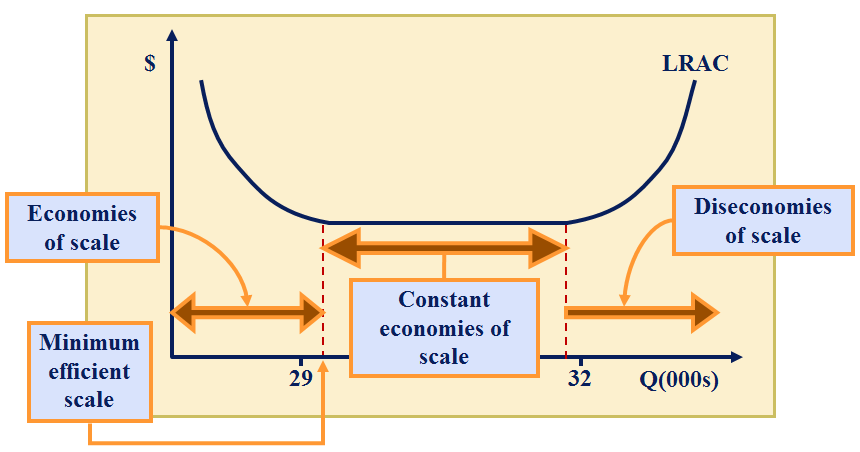
Minimum Efficient Scale (MES)
Definition: The minimum size of a firm or plant that allows it to achieve all available economies of scale
Mathematically: smallest output level at which LRAC is minimized
What do average cost curves really look like?
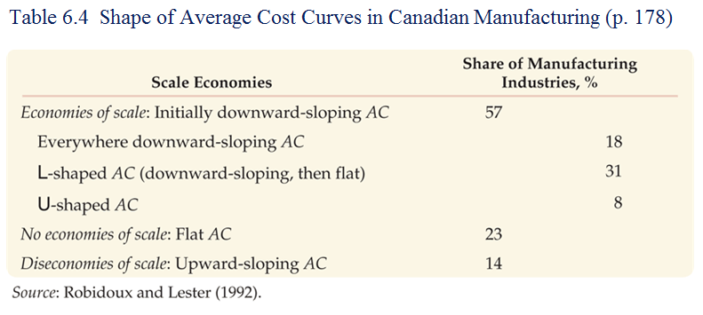
We often can’t estimate what we don’t observe – some L-shaped AC curves likely slope up at some output level, but we don’t observe firms operating in that region
Liquid Costs: Costs of Beer and Oil

BEER: Constant returns to scale in the long-run. But stuck with existing capital in short run. (p181 in textbook)
Liquid Costs: Costs of Beer and Oil

OIL: Long run decreasing returns to scale if can build larger diameter pipes.
Changes to Long Run Costs
Three main factors shift long-run cost curves:
- Economies of scope
- Learning economies
- Input prices and technological change
Economies of Scope
Economies of Scope
Economies of scope are positive if:
The cost of joint production of two (or more) distinct products is
less than the cost of producing the same amount of each product
separately
i.e. C(q1,q2) < C1(q1, 0) + C2(0, q2)
Economies of Scope
Examples of products that exhibit economies of scope?
Economies of Scope
Some production processes naturally exhibit economies of scope:
-
B-Schools: BBA, MBA, PhD, EMBA
-
Lamb meat and wool; beef and leather
-
McDonald's: breakfast and lunch
- Amazon: product sales & cloud computing
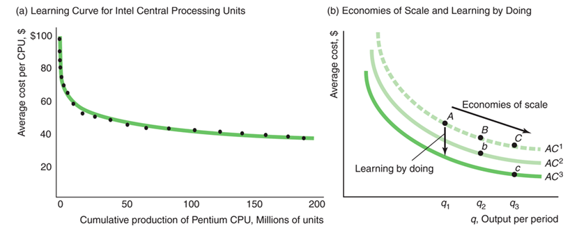
Learning Economies
Learning vs. Economies of Scale
Learning by doing for Intel (see text p. 182)
Technological Change
Permanent changes in the price of key inputs will shift long-term cost curves up or down.
-
Example: microprocessors in the computer industry
Technological change makes new combinations of inputs possible, leading to lower production costs.
Example: better logistics lead to more efficient equipment use in the trucking industry.
Regulatory change can affect production costs.
Example: emission standards and pollution permitsCost Fundamentals: Key Topics
- An opportunity cost is the implicit cost associated with using a resource in a particular endeavor
- A sunk cost is an expenditure that once made cannot be recovered
- Total economic cost includes opportunity costs and disregards sunk costs
- Average cost is total economic cost divided by output
- Marginal cost is the change in total economic cost to produce one more unit of output
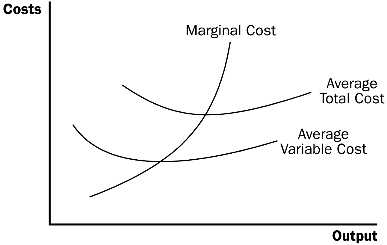
Cost Fundamentals: Key Topics
The short run is the period within which firms cannot modify the size of their facilities. Because of this, some costs are fixed in the short run.
The “Law of Diminishing Returns” says that in the short run, average costs (variable and total) must at some point increase
Cost Fundamentals: Key Topics
We care about the long run average cost curve because it tells us efficient plant sizes
Economies of scale exist when one gets more than an x% increase in output from increasing all inputs (labor, materials, capital and equipment) by x%
Competitive Markets
Perfect Competition
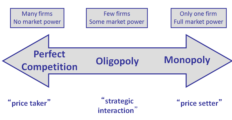
Competitive Market
Characteristics of a perfectly competitive market:- The goods offered for sale are all exactly the same.
- The buyers and sellers are so numerous that no single buyer or seller can impact the price.
- Easy to enter and exit.
- All market participants have good information.
When this is true, buyers and sellers are said to be price takers.
Can you think of examples of markets that are perfectly competitive?
Competitive Markets
Demand in competitive markets:
No one will buy your product if you raise your price above the going rate.
But--you can sell as much as you want at the current price without affecting the price.
What would the demand curve look like in this scenario?
Competitive Market
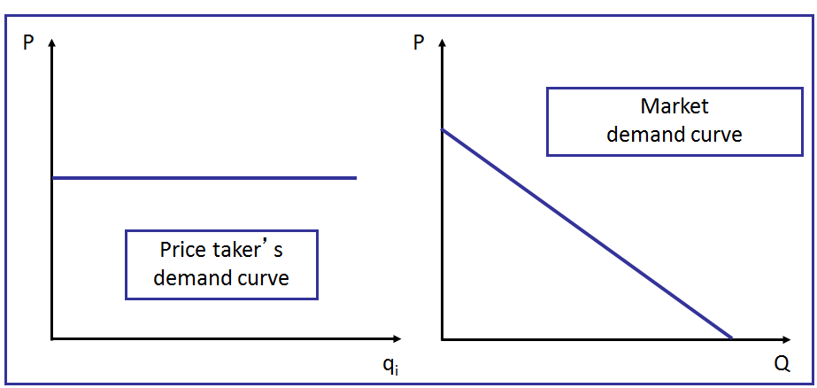
First graph measured in 100s... second graph measured in billions.
Competitive Market
Recall:
Total Revenue = Price x Quantity.
If firms are in a perfectly competitive market, how can they change their total revenue?
Competitive Markets
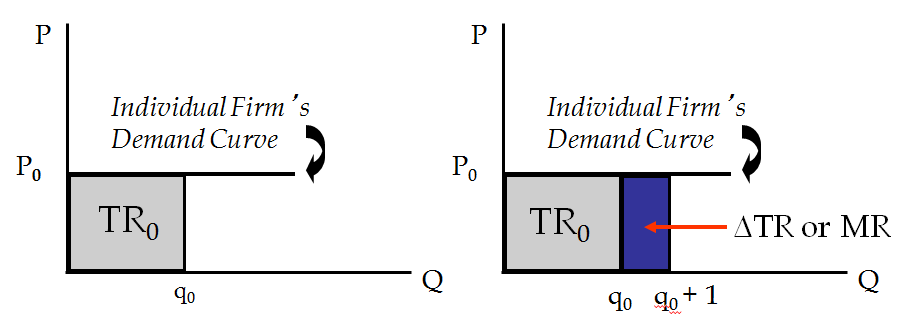
In a competitive market, selling one more unit of revenue doesn't affect the price.
Competitive Market
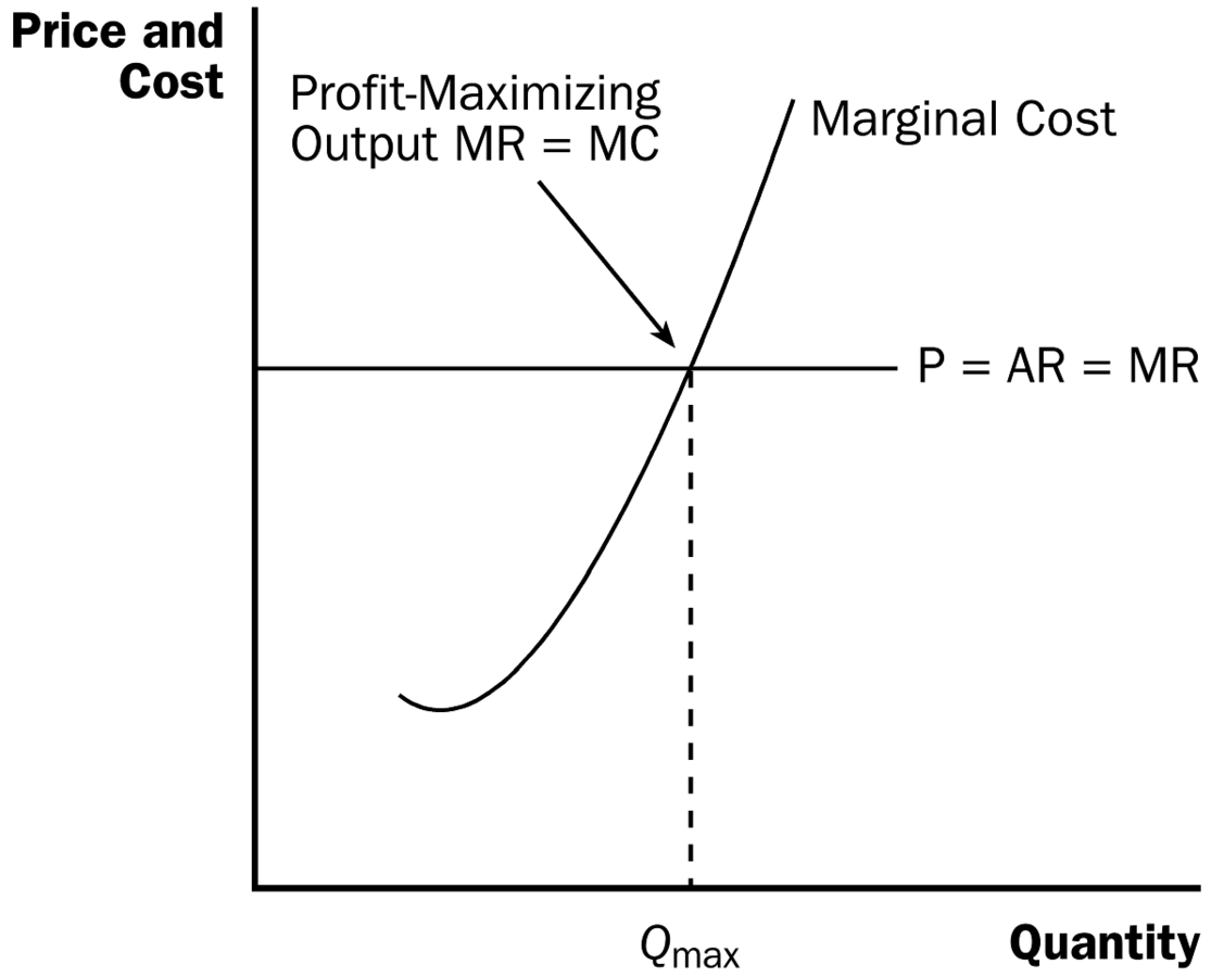
Recall:
When marginal revenue > marginal cost, profit is increasing.
=> Firms want to produce more.
When marginal revenue < marginal cost, profit is decreasing.
=> Firms want to produce less.
Profit is maximized at MC=MR.
In the competitive scenario, this occurs when MC=Price.Competitive Markets
Competitive Markets
Competitive Markets
Competitive Markets
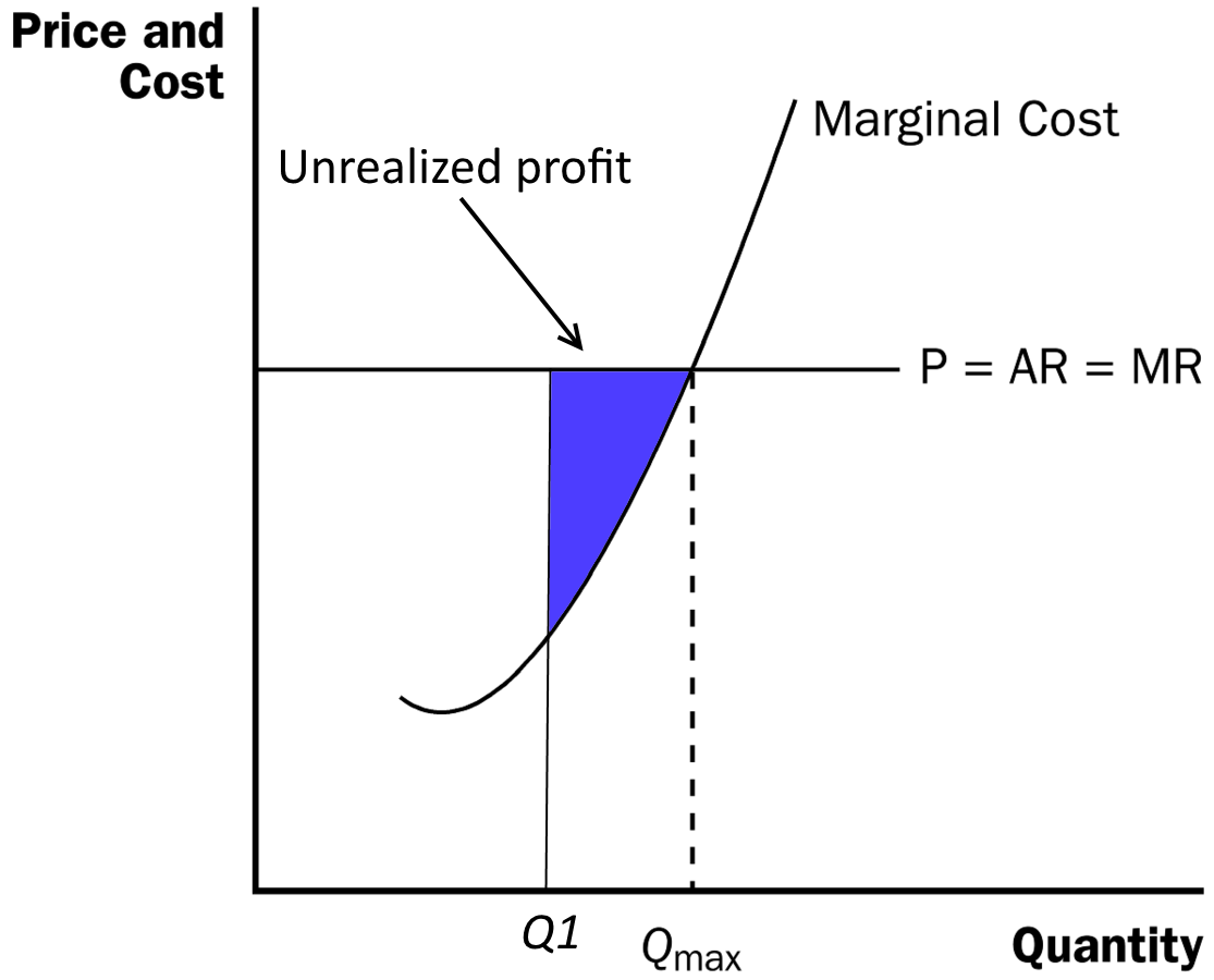
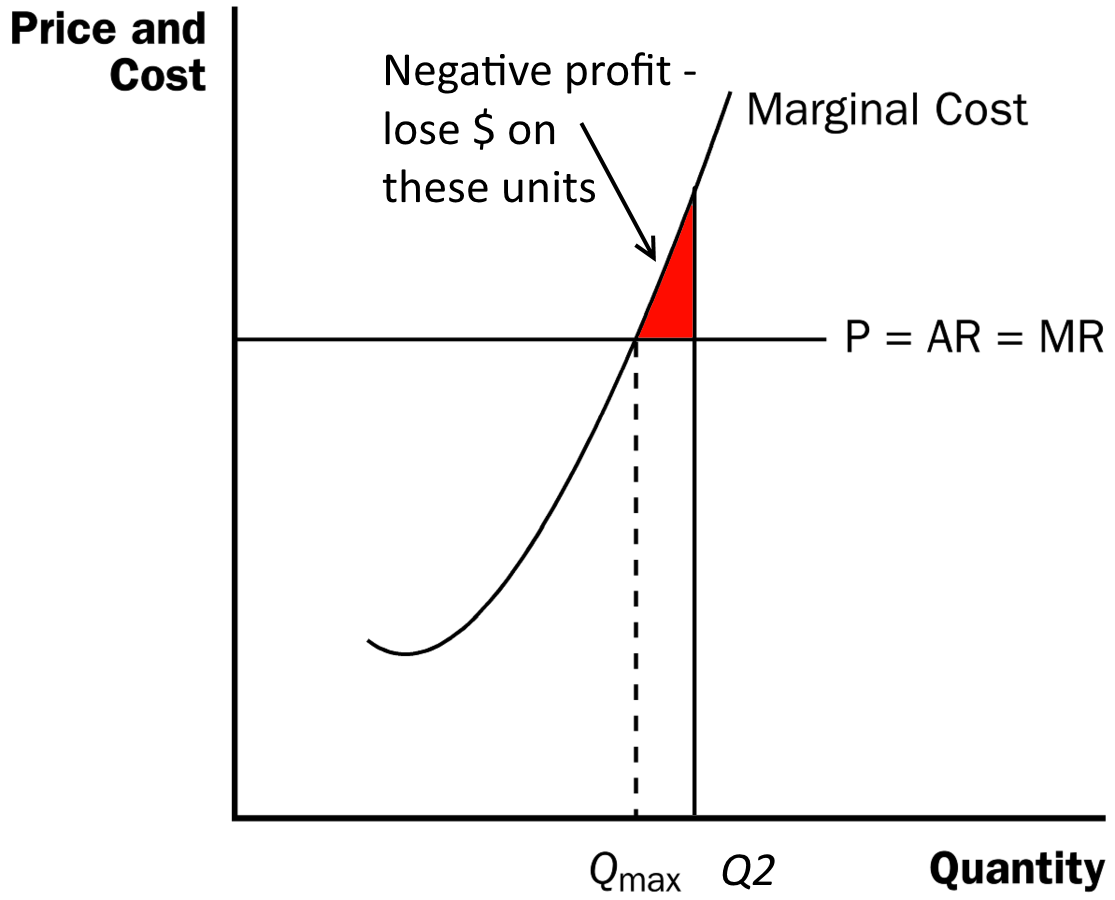
Profits are maximized where MC=P.
Competitive Markets
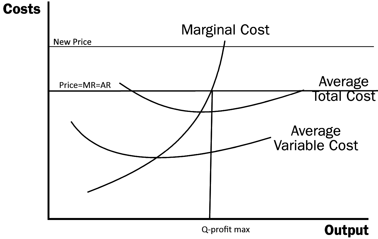
Now price goes up--what happens to quantity? Profit?
Competitive Markets
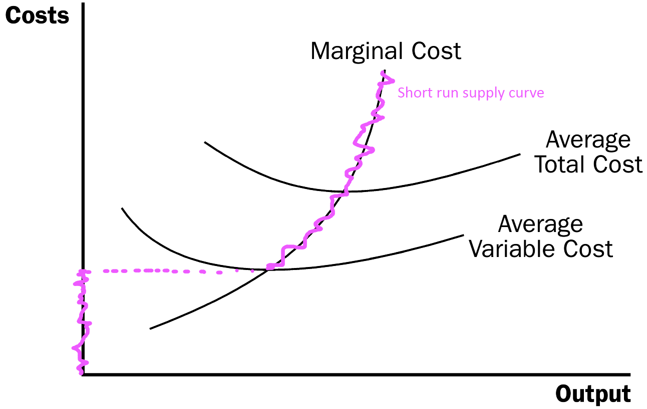
Imagine price goes down a little bit--how do you find the new quantity? What is another name for the marginal cost curve?
Competitive Market
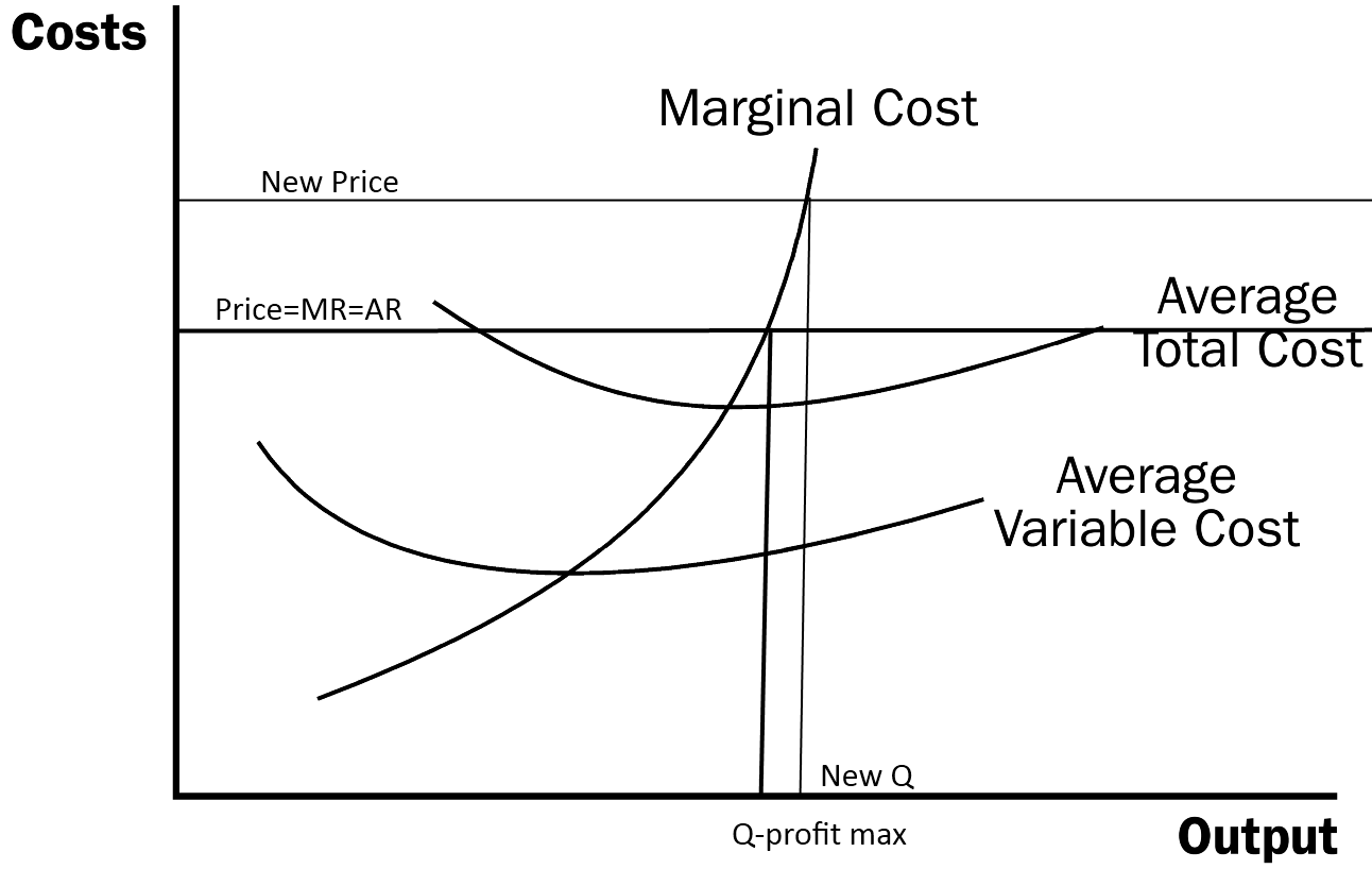
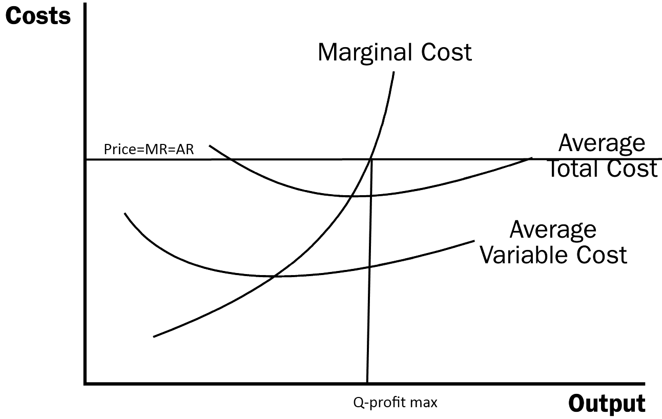
Marginal cost gives the relationship between the price and the quantity that firms want to produce. In other words, MC is the short run supply curve.
Marginal Cost
We can use our insight into the role of marginal cost in determining the short run supply to make predictions--if you know the shape of the MC curve, you know what short run supply looks like!
Competitive Markets
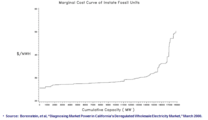
Actual marginal costs of producing a MWH.
Marginal Cost
California energy crisis--2000-2001
- Thinking about supply as directly related to marginal cost helps us make predictions.
- Large swings in price are predictable when short-run MC is sharply increasing
Competitive Markets
A chemical firm is producing 100 units of output with MC = $18, AVC
= $17, and ATC = $19. The prevailing price of the product in the
market is $18.50. There are many substitutes for this firm’s product,
so that the quantity it would sell would fall dramatically if it tried
to raise its price. To maximize short-run profits (or minimize
short-run losses if that is the best the firm can do) the firm should:
-
increase the selling price to some point above $19
-
increase its output until MC equals $18.50
-
shut down production in the short-run since it is losing money
- reduce its output so as to lower MC, AVC, and ATC and thereby earn an economic profit
Competitive Markets
“Diesel Prices are Bringing Some Trucks to a Standstill,” LA Times, 3/15/04
What type of cost does diesel represent to truckers?
How does the increase in diesel prices affect the cost curves of a typical long haul trucker?Competitive Markets
Data for John Telles:
Revenue
$1.00/mile
Costs
Fuel: $0.36/mile
Other op. expenses: $0.65/mile
Does it make sense for him to shut down?
Competitive Markets
Remember the shut down rule:
Shut down if P < AVC.
Competitive Markets
Where is the short-run supply curve?
Competitive Market
(while conceptually important, we usually will not draw the part of the supply curve that goes along the vertical axis)
Competitive Market
What will shift the short-run supply curve?
Competitive Market
We've discussed the decision making process of a single firm. But, we can also aggregate firms up to the market level.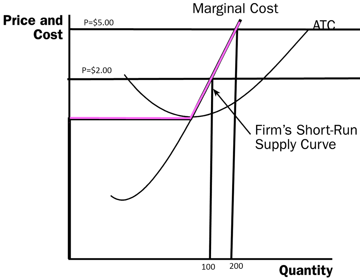
Competitive Market
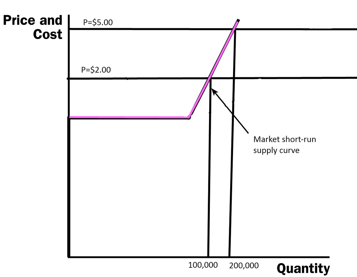
The supply in the market reflects the marginal costs of all the individual firms that comprise the market.
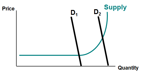
Competitive Markets
On this graph (the graph of the market supply curve), what will the demand curve look like?
Competitive Market
Let's think back to our supply and demand model:
Competitive Market
Competitive Markets
Competitive Markets
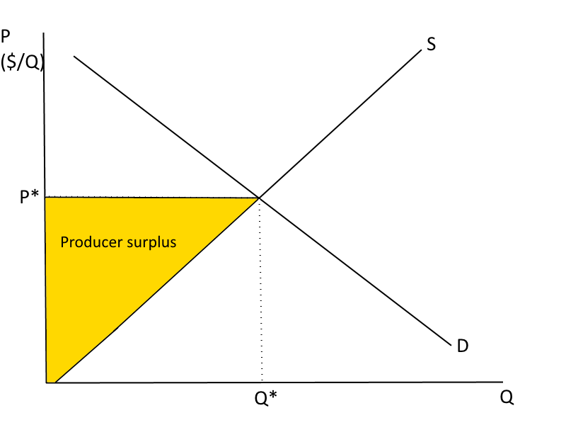
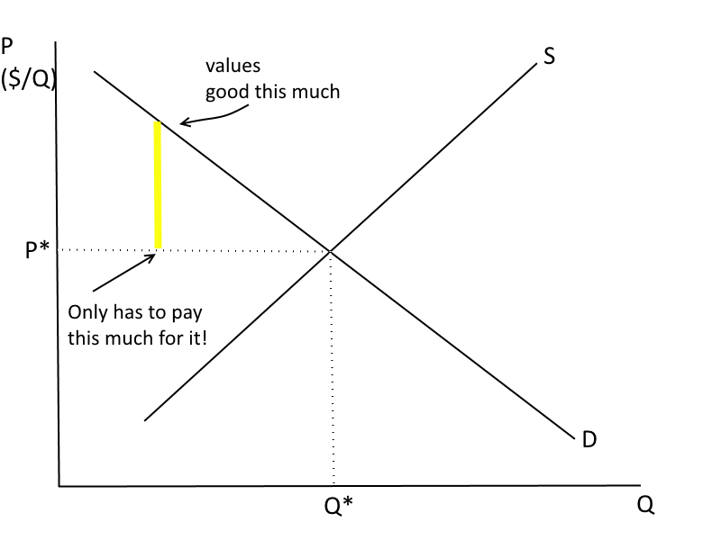
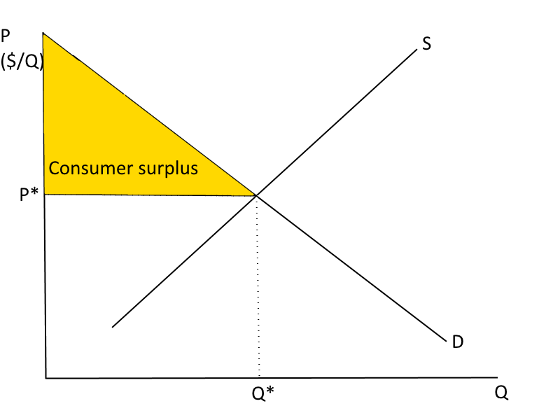
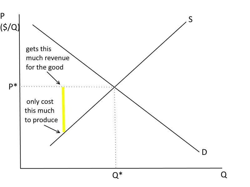
Analogous to consumer surplus--"willingness to supply."
Competitive Markets
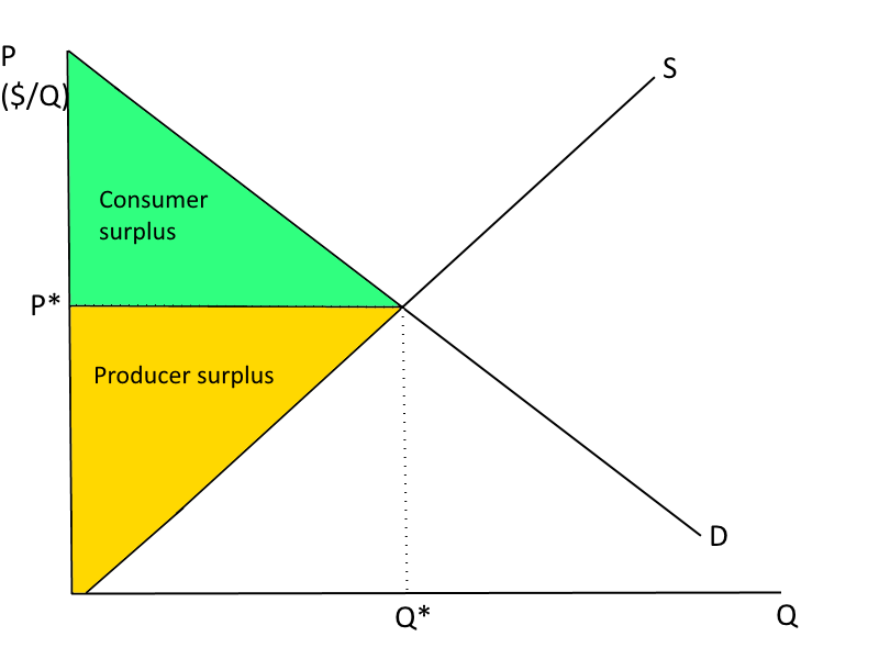
Total surplus (or total "welfare") is consumer+producer surplus.
Competitive Markets
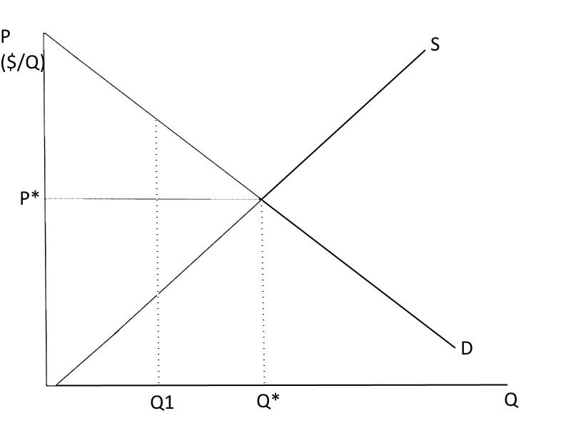
Say we are producing at Q1. Where is total surplus? What happens to total surplus when we increase production?
Competitive Markets
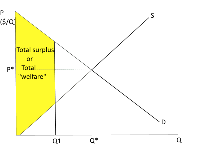
Total surplus at Q1
Competitive Markets
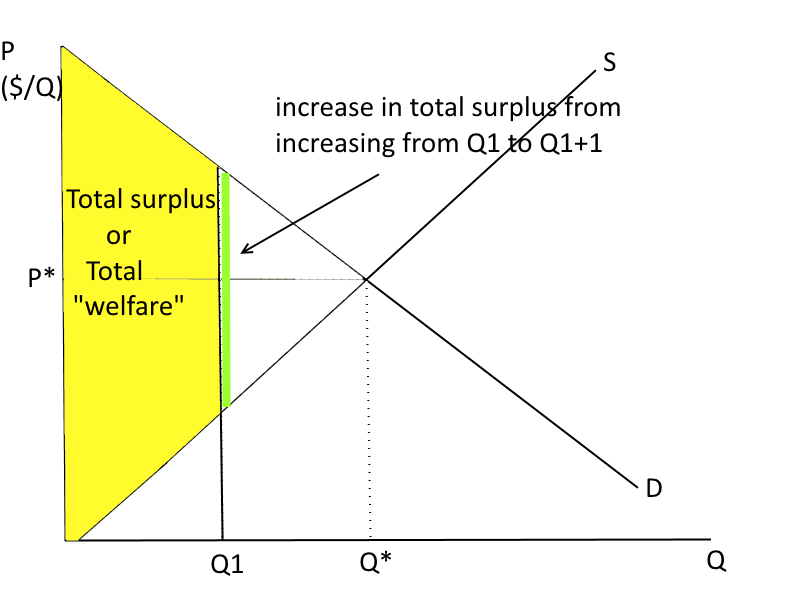
Where is total surplus maximized?
Competitive Markets
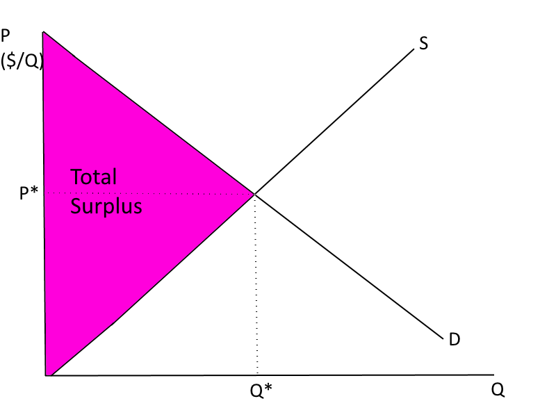
Total surplus is maximized at the market equilibrium.
Competitive Markets
Consumers and producers in a competitive market -- acting only on their own self interest -- will drive the market to the price and quantity that maximizes the total surplus.
Competitive Markets
Given the following information:
Market Demand: P = 1000 - 0.25Q
Market Supply: P = 300 + 0.1Q
TC for each firm: TC = 100 + 300q + 5q^2
MC for each firm = 300+10q
What will be the short-run market equilibrium P, Q, CS, PS.
What will be individual firm quantity and profit, and the
equilibrium number of firms in the market? Illustrate the firm and
market equilibrium.
Next Time:
THURSDAY Feb. 5
Textbook: Ch. 2.5; pp. 265 – 268; Ch. 9 intro, 9.1 – 9.4; Ch. 8.4; Ch. 16 intro & Ch. 16.1
We will also do an in-class simulation.
Exercise Solutions
Exercise 1:
P = 1000 - 0.25Q ; S: P = 300 + 0.1QTC = 100 + 300q + 5q2 so MC = dTC/dq = 300 + 10q
Short-run market equilibrium: Demand = Supply
1000 - 0.25Q = 300 + 0.1Q
Q* = 2000, P* = $500
At the firm level:
P = MC, 500 = 300 + 10q, q* = 20
Profit = TR - TC = 500(20) - [100 + 300(20) + 5(20)2] = $1,900, so this industry is not currently in long-run equilibrium since profits are positive
# firms = Q/q = 2000/20 = 100, CS = 500 * 2000 * 0.5 = 500,000 , PS = 200 * 2000 * 0.5 = 200,000
Lecture 7
By umich


