


Vidhi Lalchand
Postdoctoral Fellow, Broad and MIT
Vidhi Lalchand
MIT Kavli Institute for Astrophysics and Space Research
22-03-2023
Research Seminar
- Thomas Garrity
Gaussian processes as a "function" learning paradigm.
Regression with GPs: Both inputs \((X)\) and outputs \( (Y)\) are observed.
Latent Variable Modelling with GP: Only outputs \( (Y)\) are observed.
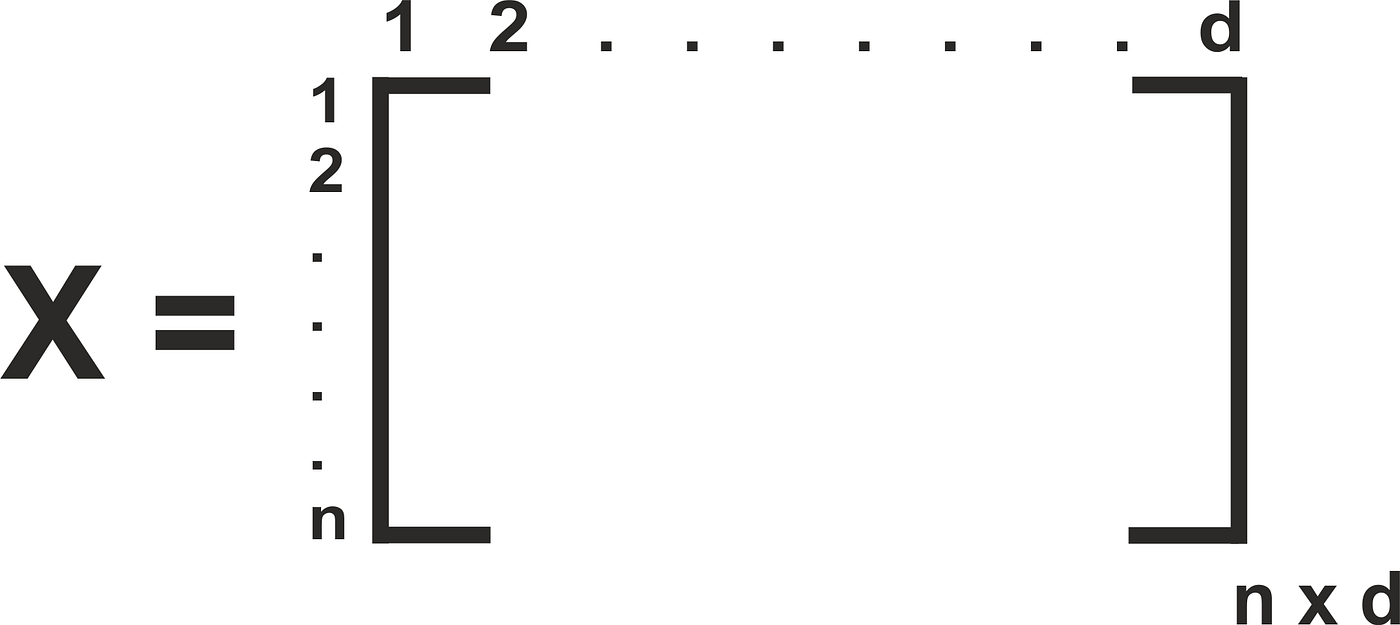
Without loss of generality, we are going to assume \( X \equiv \{\bm{x}_{n}\}_{n=1}^{N}, X \in \mathbb{R}^{N \times D}\) and \( Y \equiv \{\bm{y}_{n}\}_{n=1}^{N}, Y \in \mathbb{R}^{N \times 1}\)
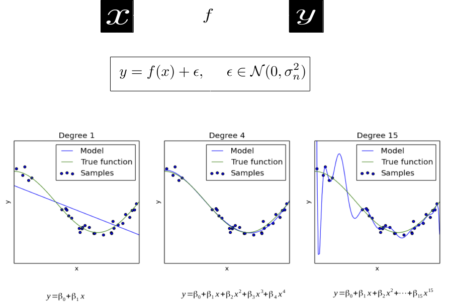
Hot take: Almost all machine learning comes down to modelling functions.
\(x \in \mathbb{R}^{d}\)
Model selection is a hard problem!
What if we were not forced to decide the complexity of \( f\) at the outset. What if \(f\) could calibrate its complexity on the fly as it sees the data - this is precisely called non-parameteric learning.
Gaussian Processes
Gaussian processes are a powerful non-parametric paradigm for performing state-of-the-art regression.
We need to understand the notion of distribution over functions.
A continuous function \( f \) on the real domain \( \mathbb{R}^{d} \), can be thought of as an infinitely long vector evaluated at some index set \( [x_{1}, x_{2}, ......]\).
\( [f(x_{1}), f(x_{2}), f(x_{3}),.......]\)
Gaussian processes are probability distributions over functions!
Interpretation of functions
Sticking point: We cannot represent infinite dimensional vectors on a computer....true, but bear with me.
\(m(x)\) is a mean function.
\(k(x, x')\) is a covariance function.
What is a GP?
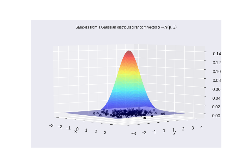
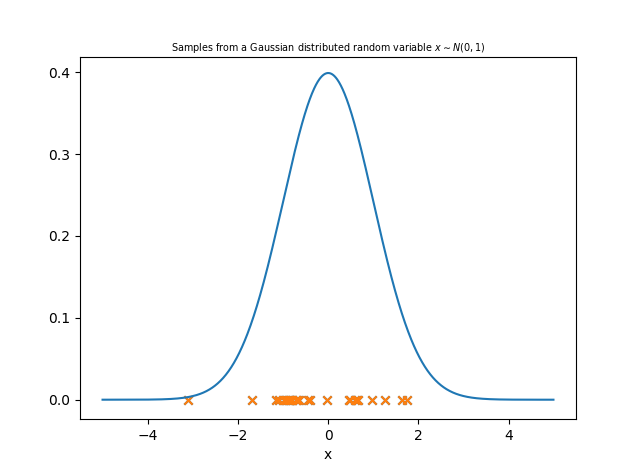
The most intuitive way of understanding GPs is understanding the correspondence between Gaussian distributions and Gaussian processes.
What is a GP?
A sample from a \(k\)-dimensional Gaussian \( \mathbf{x} \sim \mathcal{N}(\mu, \Sigma) \) is a vector of size \(k\). $$ \mathbf{x} = [x_{1}, \ldots, x_{k}] $$
The mathematical crux of a GP is that \( [f(x_{1}), f(x_{2}), f(x_{3}),....., f(x_{n})]\) is just a N-dimensional multivariate Gaussian \( \mathcal{N}(\mu, K) \).
A GP is an infinite dimensional analogue of a Gaussian distribution \( \rightarrow \) a sample from it is a vector of infinite length?
But at any given point, we only need to represent our function \( f(x) \) at a finite index set \( \mathcal{X} = [x_{1},\ldots, x_{500}]\). So we are interested in our long function vector \( [f(x_{1}), f(x_{2}), f(x_{3}),....., f(x_{500})]\).
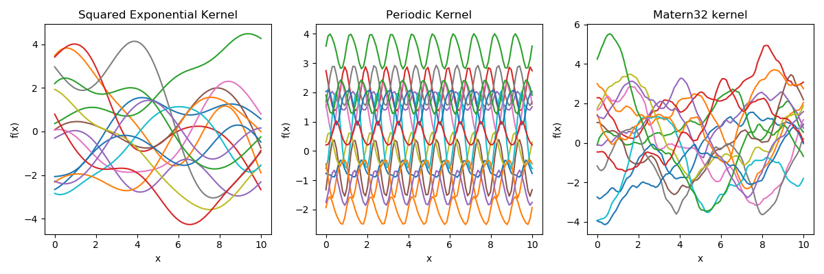
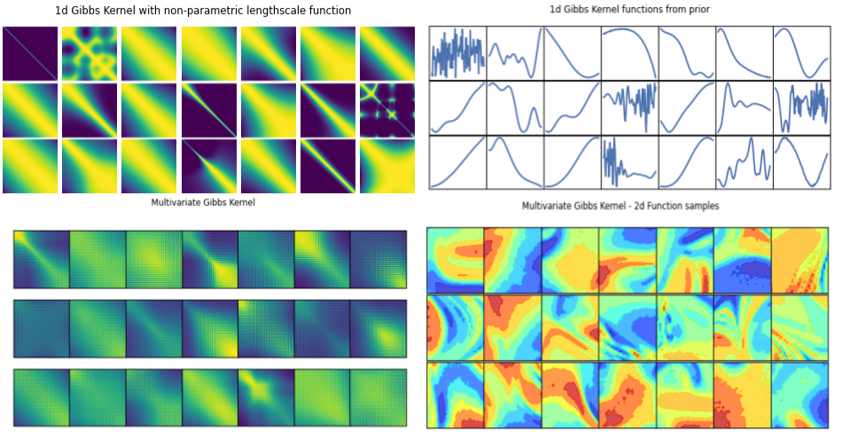
Function samples from a GP
The kernel function \( k(x,x')\) is the heart of a GP, it controls all of the inductive biases in our function space like shape, periodicity, smoothness.
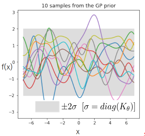
prior over functions \( \rightarrow \)
Sample draws from a zero mean GP prior under different kernel functions.
In reality, they are just draws from a multivariate Gaussian \( \mathcal{N}(0, K)\) where the covariance matrix has been evaluated by applying the kernel function to all pairs of data points.
Infinite dimensional prior:
\(f(x) \sim \mathcal{GP}(m(x), k_{\theta}(x,x^{\prime})) \)
\(f(X) \sim \mathcal{N}(m(X), K_{X})\)
For a finite set of points, \( X \):
\( k_{\theta}(x,x^{\prime})\) encodes the support and inductive biases in function space.
Gaussian Process Regression
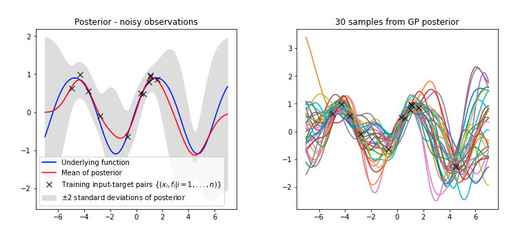
How do we fit functions to noisy data with GPs?
1. Given some noisy data \( \bm{y} = \lbrace{y_{i}}\rbrace_{i=1}^{N} \) at \( X = \{ x_{i}\}_{i=1}^N\) input locations.
2. You believe your data comes from a function \( f\) corrupted by Gaussian noise.
$$ \bm{y} = f(X) + \epsilon, \hspace{10pt} \epsilon \sim \mathcal{N}(0, \sigma^{2})$$
Data Likelihood: \( \hspace{10pt} y|f \sim \mathcal{N}(f(x), \sigma^{2}) \)
Prior over functions: \( f|\theta \sim \mathcal{GP}(0, k_{\theta}) \)
(The choice of kernel function \( k_{\theta}\) controls how your functions space looks.)
.....but we still need to fit the kernel hyperparameters \( \theta\)
Learning Step:
Learning in Gaussian process models occurs through the maximisation of the marginal likelihood w.r.t the kernel hyperparameters.
Data likelihood
Prior
Denominator of Bayes Rule
Learning in a GP
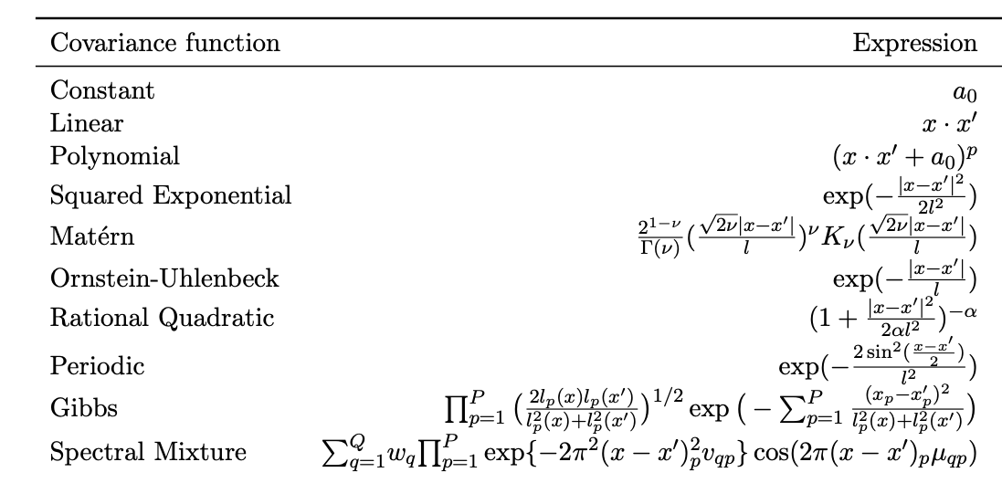
Popular Kernels
Usually, the user picks one on the basis of prior knowledge.
Each kernel depends on some hyperparameters \( \theta\), which are tuned in the training step.
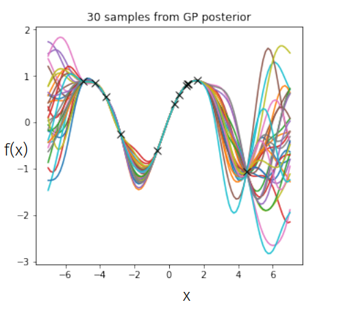
Predictions in a GP
We want to infer latent function values \(f_{*}\) at any arbitrary input locations \( X_{*} \), so in a distribution sense we want,
$$ p(f_{*}|X_{*}, y, \theta) $$
Posterior Predictive Distribution
The predictive posterior is closed form (because we are operating a world of Gaussians):
Joint
Conditional
can be derived using symmetry arguments
Predictions in a GP
Joint
Conditional
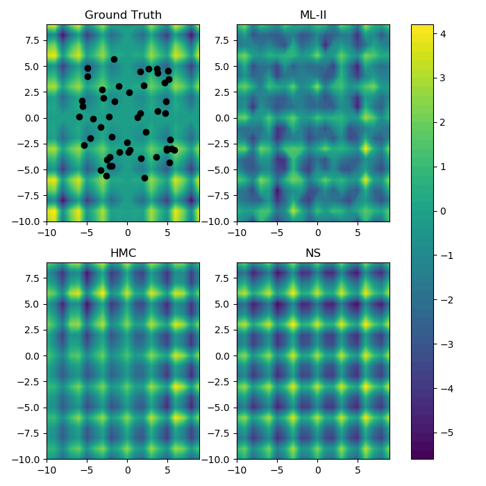
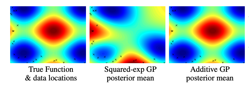
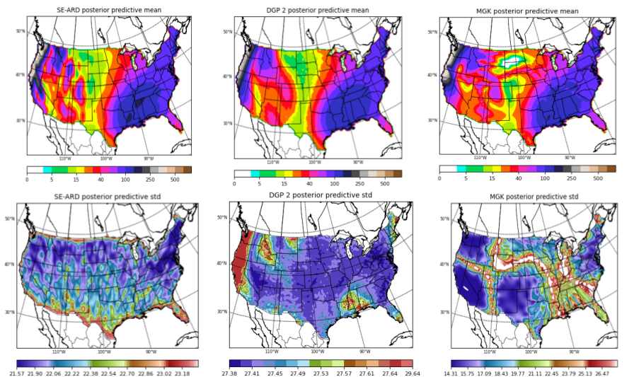
Examples of GP Regression
Examples of GP Regression
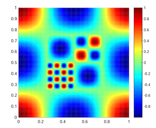
Ground Truth
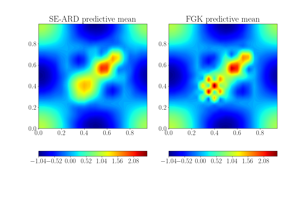
Reconstruction
Examples of GP Regression
Gaussian processes can also be used in contexts where the observations are a gigantic data matrix \( Y \equiv \{ y_{n}\}_{n=1}^{N}, y_{n} \in \mathbb{R}^{D}\). \(D\) can be pretty big \(\approx 1000s\).
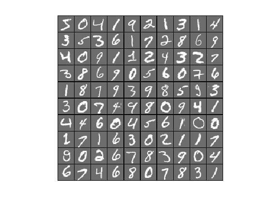
Imagine a stack of images, where each image has been flattened into a vector of pixels and stacked together rowise in a matrix.
28
28
n = number of images
d = 784
N x D
The Gaussian process bridge
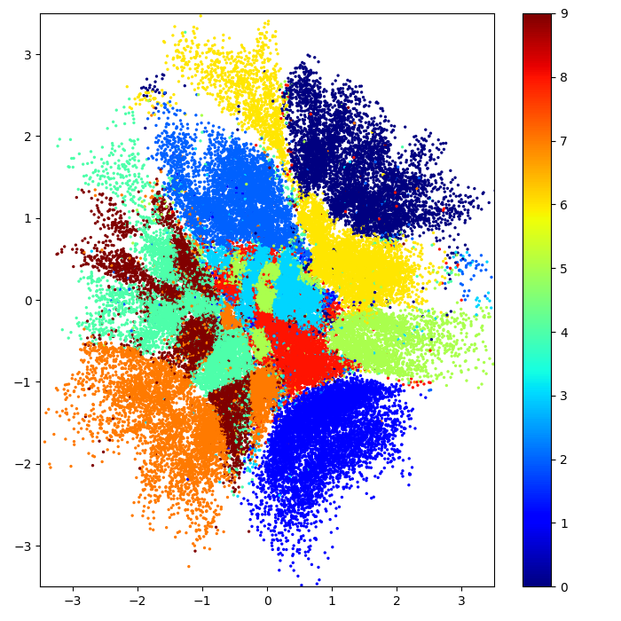
2d latent space
High-dimensional data space
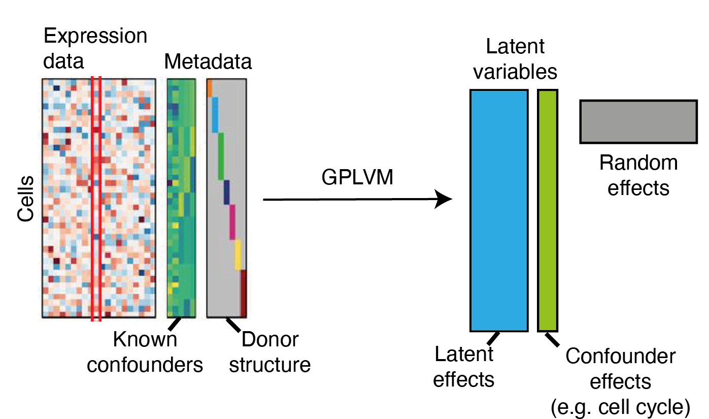
Schematic of a Gaussian process Latent Variable Model
. . .
. . .
. . .
N
D
Structure / clustering in latent space can reveal insights into the high-dimensional data - for instance, which points are similar.
each cluster is a digit (coloured by labels)
\( Z \in \mathbb{R}^{N \times Q}\)
\( F \in \mathbb{R}^{N \times D}\)
\( Y \in \mathbb{R}^{N \times D} (= F + noise)\)
Mathematical set-up
Data Likelihood:
Prior structure:
The data are stacked row-wise but modelled column-wise, each column with a GP.
\(Z\)
\(z_{n}\)
Mathematical set-up
The data are stacked row-wise but modelled column-wise, each column with a GP.
\(Z\)
\(z_{n}\)
Optimisation objective:
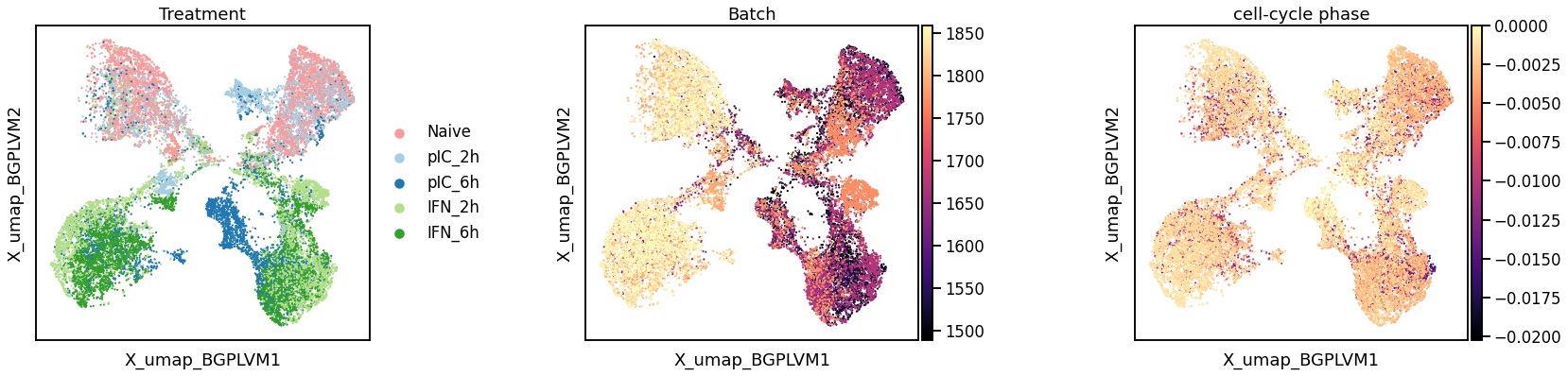
Treatment
Latent batch effect
Cell cycle phase
Disentanglement of cell cycle and treatment effects
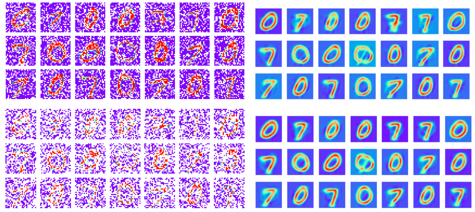
Robust to Missing Data: MNIST Reconstruction
30%
60%
Robust to Missing Data: Motion Capture
Thank you!
vr308@cam.ac.uk
@VRLalchand
By Vidhi Lalchand


