Modelling Cancer Drug Synergy Surfaces with Gaussian Processes

Vidhi Lalchand

14-11-2025

Drug-synergy modelling through dose-response surfaces

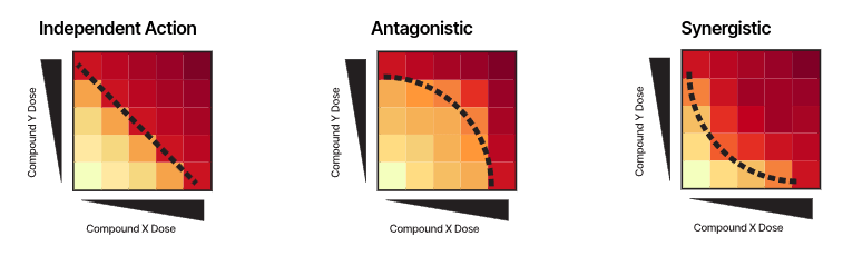
The nature of a drug combination, as synergistic, antagonistic or non-interacting, is usually studied by in-vitro dose–response experiments on cancer cell lines, through e.g. a cell viability assay.

https://theprismlab.org/white-papers/multiplexed-cancer-cell-line-combination-screening-using-prism

Combination therapies are routinely used in cancer care, as monotherapies are rarely effective.
However, which combinations would benefit cancer patients is largely unknown.
Studies that measure candidate combinations (of drugs) across many cancer cell lines simultaneously can help support combinations research [PRISM Lab].

Drug-synergy modelling: Bliss model of independence

https://theprismlab.org/white-papers/multiplexed-cancer-cell-line-combination-screening-using-prism

The Bliss model assumes that the two drugs X and Y act independently to achieve their effects.

$E_A$ : The probability of drug $A$ killing a cell.
$E_B$ : The probability of drug $B$ killing a cell.
The probability of neither drug killing a cell is:
$E_A) \cdot (1 - E_B).$
Therefore, the expected viability $V_{XY}$ is, $VABV_{ABV$
$VAB=VA⋅VB,V_{AB} = V_A \cdot V_B,$

Observed Results:

If $Vobs=0.2V_{\text{obs}} = 0.2$ : Synergy (fewer cells survive than expected).
If $Vobs=0.3V_{\text{obs}} = 0.3$ : Additivity (matches expected survival).
If $Vobs=0.4V_{\text{obs}} = 0.4$ : Antagonism (more cells survive than expected).

$V_{X} = 0.5$ and $V_{Y} =0.6$

$V_{XY} = 0.3$

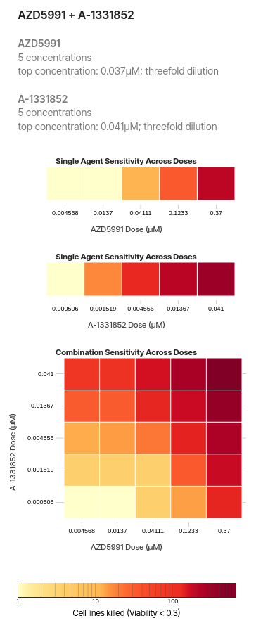
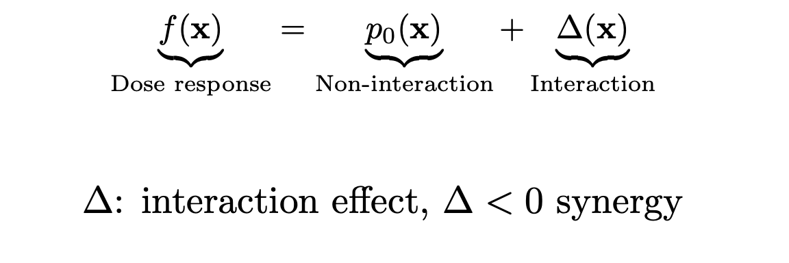
Drug-synergy modelling through dose-response surfaces

Bliss independence

Non-linear effect

I use Gaussian processes to model this non-linear effect

What is a GP?

A sample from a $k$-dimensional Gaussian $ \mathbf{x} \sim \mathcal{N}(\mu, \Sigma) $ is a vector of size $k$. $$ \mathbf{x} = [x_{1}, \ldots, x_{k}] $$

The mathematical crux of a GP is that $ \textbf{f} \equiv [f(x_{1}), f(x_{2}), f(x_{3}),....., f(x_{N})]$ is just a N-dimensional multivariate Gaussian.

\begin{bmatrix} f_{1} \\ \vdots\\ f_{499} \\ f_{500} \end{bmatrix} \sim \mathcal{N}\left(\begin{bmatrix} m(x_{1}) \\ \vdots\\ m(x_{499}) \\ m(x_{500}) \\ \end{bmatrix}, \begin{bmatrix} k(x_{1}, x_{1}) & \ldots & \ldots k(x_{1}, k_{500}) \\ \vdots & \ddots &\vdots \\ \vdots & \ddots & \vdots \\ k(x_{500}, x_{1}) & \ldots & \ldots k(x_{500}, k_{500}) \\ \end{bmatrix} \right)

A GP is an infinite dimensional analogue of a Gaussian distribution $ \rightarrow $ a sample from it is a vector of infinite length?

f(x) \sim \mathcal{GP}(m(x),k(x, x^{\prime}))

But at any given point, we only need to represent our function $ f(x) $ at a finite index set $ \mathcal{I} = [x_{1},\ldots, x_{500}]$. So we are interested in our 500 dimensional function vector $ [f(x_{1}), f(x_{2}), f(x_{3}),....., f(x_{500})]$.

p(f_{1}, f_{2}, \ldots, f_{N}) = \int\ldots \int p(f_{1}, f_{2}, \ldots, \ldots) df_{{j} (j \notin \mathcal{I})}

Marginalising function values corresponding to inputs not in our index set.

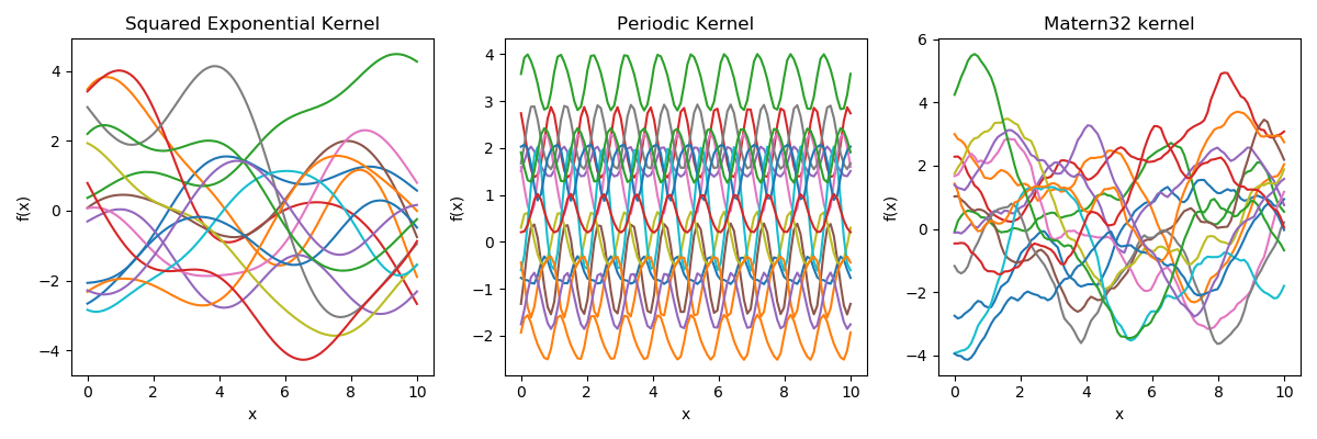
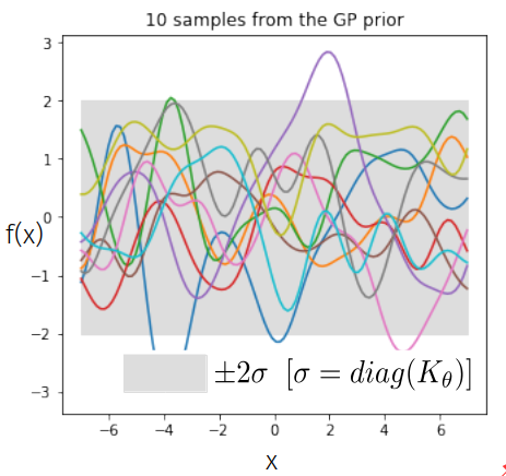
Samples from a GP

f(x) \sim \mathcal{GP}(m(x),k(x, x^{\prime}))

prior over functions $ \rightarrow $

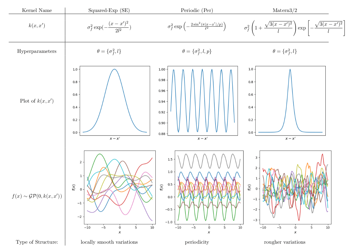
Sample draws from a zero mean GP prior under different kernel functions.

In reality, they are just draws from a multivariate Gaussian $ \mathcal{N}(0, K)$ where the covariance matrix has been evaluated by applying the kernel function to all pairs of data points.

Rigorous definition: $ f$ is a GP if for any finite subset $\{x_{1}, \ldots, x_{n}\} \subset \mathcal{X}$, the marginal distribution of function values $ p(\textbf{f})$ is Gaussian.

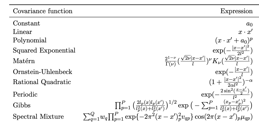
Popular Kernels

Usually, the user picks one on the basis of prior knowledge.

Each kernel depends on some hyperparameters $ \theta$, which are tuned in the training step.

The kernel function $ k(x,x')$ is the heart of a GP, it controls all of the inductive biases in our function space like shape, periodicity, smoothness.

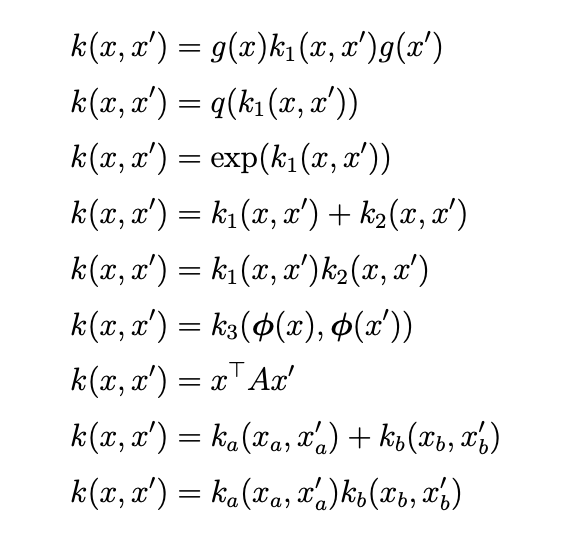
Closed operations on kernels

Stationary kernels

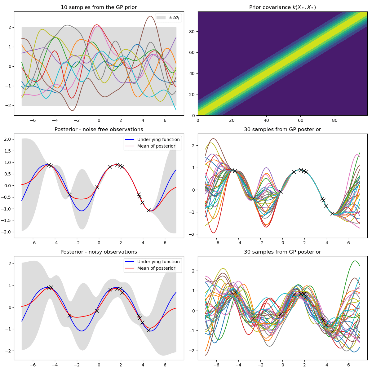
Gaussian Process Regression

How do we fit functions to noisy data with GPs?

1. Given some noisy data $ \bm{y} = \lbrace{y_{i}}\rbrace_{i=1}^{N} $ at $ X = \{ x_{i}\}_{i=1}^N$ input locations.

2. You believe your data comes from a function $ \bm{f}$ corrupted by Gaussian noise.

$$ y_{i} = f(x_{i}) + \epsilon, \hspace{10pt} \epsilon \sim \mathcal{N}(0, \sigma^{2})$$

Data Likelihood: $ \hspace{10pt} \bm{y}|\bm{f} \sim \mathcal{N}(\bm{f}, \sigma^{2}\mathbb{I}) $

Prior over functions: $ f|\theta \sim \mathcal{GP}(0, k_{\theta}), \bm{f} \sim \mathcal{N}(\bm{0}, K_{\theta}) $

\rightarrow

\begin{aligned} \textbf{f} &\sim \mathcal{N}(0, K_{\theta}) \\ K_{i,j} &= k_{\theta}(x_{i}, x_{j}) \\ &\hspace{2mm} \forall i, j\\ \end{aligned}

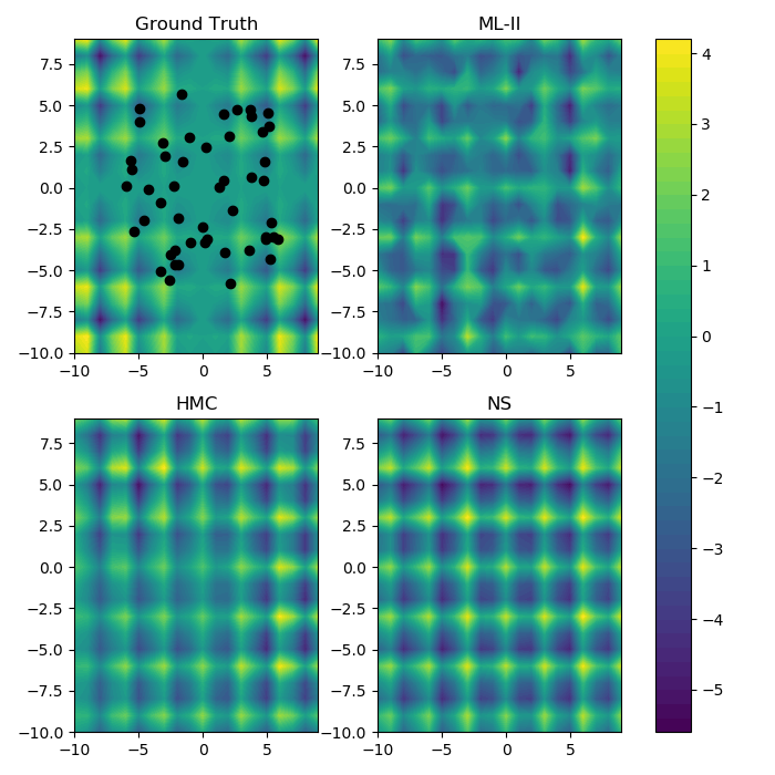
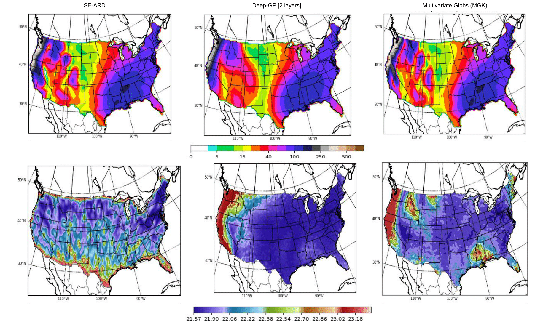
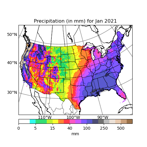
Example of fitting a 2d surface with GP regression

Multiple inference methods

Ground Truth

GPs are excellent for fitting low dimensional surfaces and adapting to the smoothness characteristics inherent in the data.

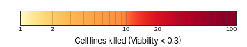
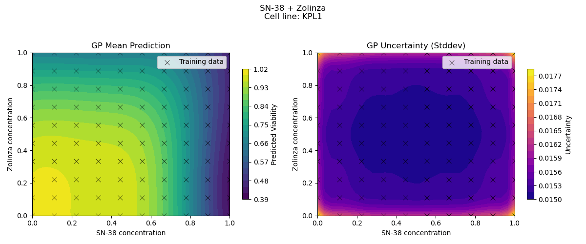
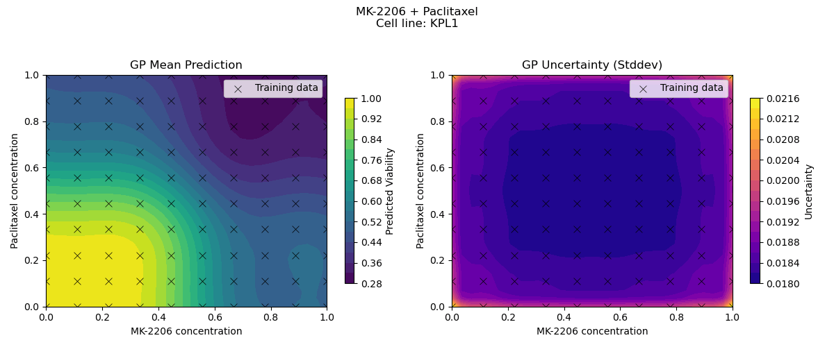
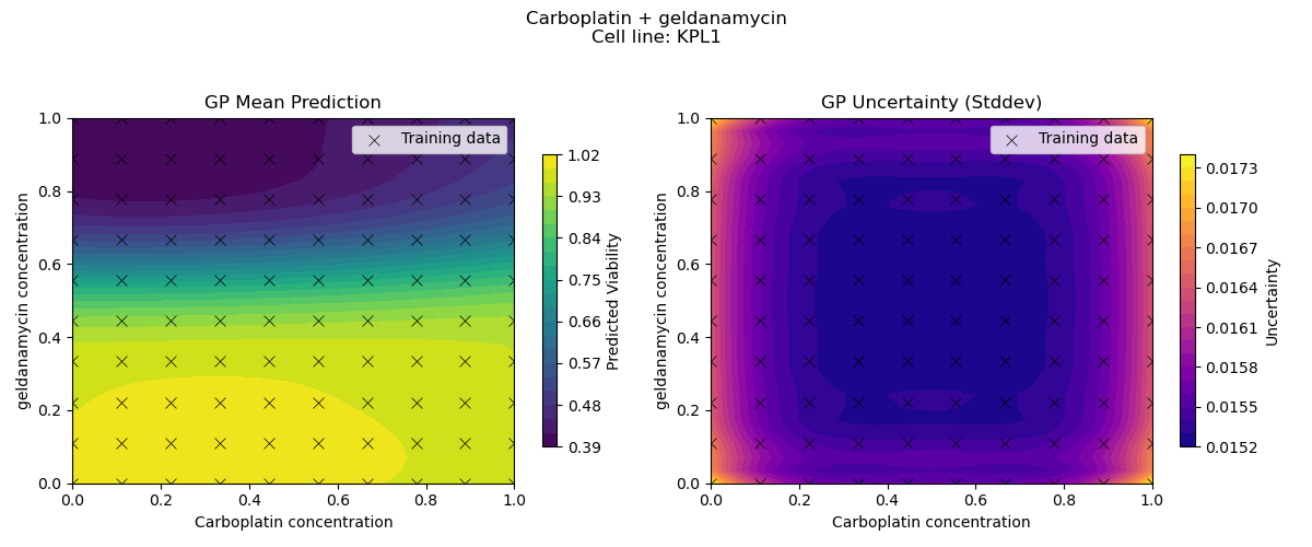
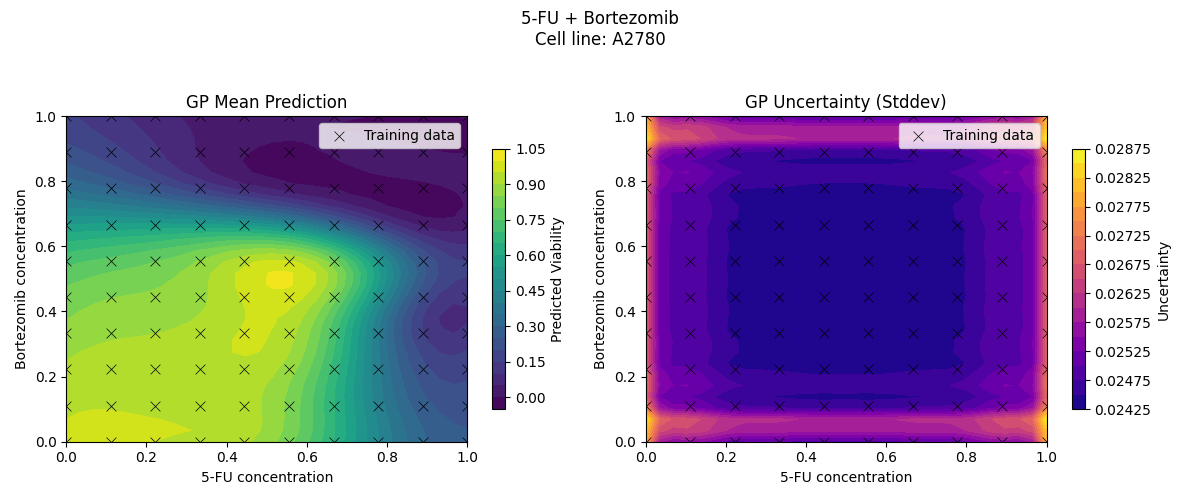
Sample drug synergy surfaces [2d fitted with a GP]

Computational Problem

Learn a model from observed drug combination viabilities

Predict a drug synergy surface for unseen chemical compounds

[For simplicity, we fix the cell-line and first try to model the variation in viabilities driven by variation in drugs]

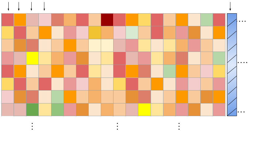
(c1, A, B)

(c1, C, D)

(c1, E, F)

(c1, X, Y)

(0, 0.11)

(0,0.22)

(0,0.33)

........

(1,1)

$N_{d}$ = 583

$N_{}$ = 100

No. of drug concentrations

No. of drug pairs.

Mathematical Framework (1/2)

\text{Define the data matrix } Y, \text{for each drug pair } p \in \{1, \dots, N\}:\\ \begin{aligned} &\text{(1) Evaluate its GP posterior mean:} && \mu_p(x_A, x_B) \text{ on a fixed } G \times G \text{ grid } X = \{ (x_A^i, x_B^j) \}_{i,j=1}^G \\[6pt] &\text{(2) Vectorize it:} && y_p = \mathrm{vec}(\mu_p) \in \mathbb{R}^{G^2} \\[6pt] &\text{(3) Stack all surfaces as columns:} && Y = [\, y_1,\, y_2,\, \ldots,\, y_N \,] \in \mathbb{R}^{G^2 \times N} \end{aligned}\\ \text{Each column of } Y \text{ corresponds to one GP mean surface (flattened)}

Y \;=\; \begin{bmatrix} | & | & | & | \\ | & | & | & | \\ \; \mathrm{vec}(\mu_{p_1}) & \mathrm{vec}(\mu_{p_2}) & \cdots & \mathrm{vec}(\mu_{p_N}) \\ | & | & | & | \\ | & | & | & | \\ \end{bmatrix} \in \mathbb{R}^{G^2 \times N}

Step 2: Find an optimal basis

Step 1:

\begin{aligned} \min_{\Phi,\,C} \| Y - \Phi C \|_F^2, \text{s.t. } \Phi^\top \Phi = I_K, \\ \text{where } \Phi \in \mathbb{R}^{G^2 \times K}\\ C \in \mathbb{R}^{K \times N} \end{aligned}

is the matrix whose columns are the shared basis functions,

is the matrix of coefficients for each drug pair, column-wise

\mu_p(x) \;\approx\; \sum_{k=1}^{K} c_{p,k} \, \phi_k(x)

Y = U \, \Sigma \, V^\top, \Phi = U_{[:,\,1:K]}, \qquad C = \Phi^\top Y = \Sigma_{1:K,\,1:K} \, V_{[:,\,1:K]}^\top

The minimisation has a closed-form solution in the form of SVD:

This guarantees the smallest reconstruction error among all orthonormal bases of size $K$

Mathematical Framework (2/2)

Interpretation

Rows of $Y$ : sampled points on the surface (shared grid).
Columns of $Y$ : drug pairs.
Columns of $Φ\Phi$ : basis functions (shared spatial patterns).
Rows of $C$ : coefficients describing how much each pattern appears in each pair.

\mu_p(x) \;\approx\; \sum_{k=1}^{K} c_{p,k} \, \phi_k(x)

Step 3: Regress on to the coefficients from the drug embeddings:

h\!\big(\psi(A,B)\big) \;\approx\; c_p

Step 4: Reconstruct surface from the predicted coefficients for each pair

For a new drug pair $p^\*$ :

You compute its drug embedding $ψ(A\*,B\*)\psi(A^\*,B^\*)$
Predict the coefficient vector $ \hat{c}_{p_{*}}$ via your regression model $h$ .
Reconstruct the full surface,

\widehat{\mu}_{p^\ast}(x) \;=\; \sum_{k=1}^{K} \widehat{c}_{p^\ast,k} \, \phi_k(x)

Note: Choice of drug embeddings should be permutation invariant

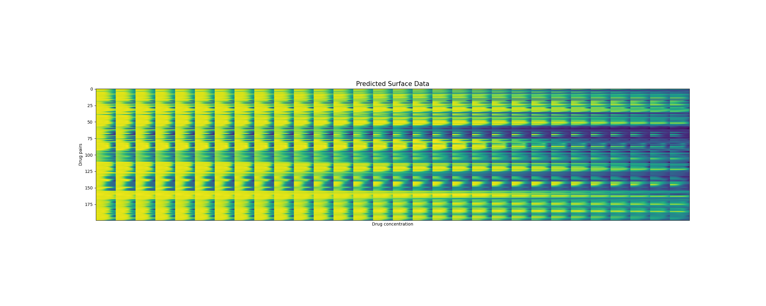
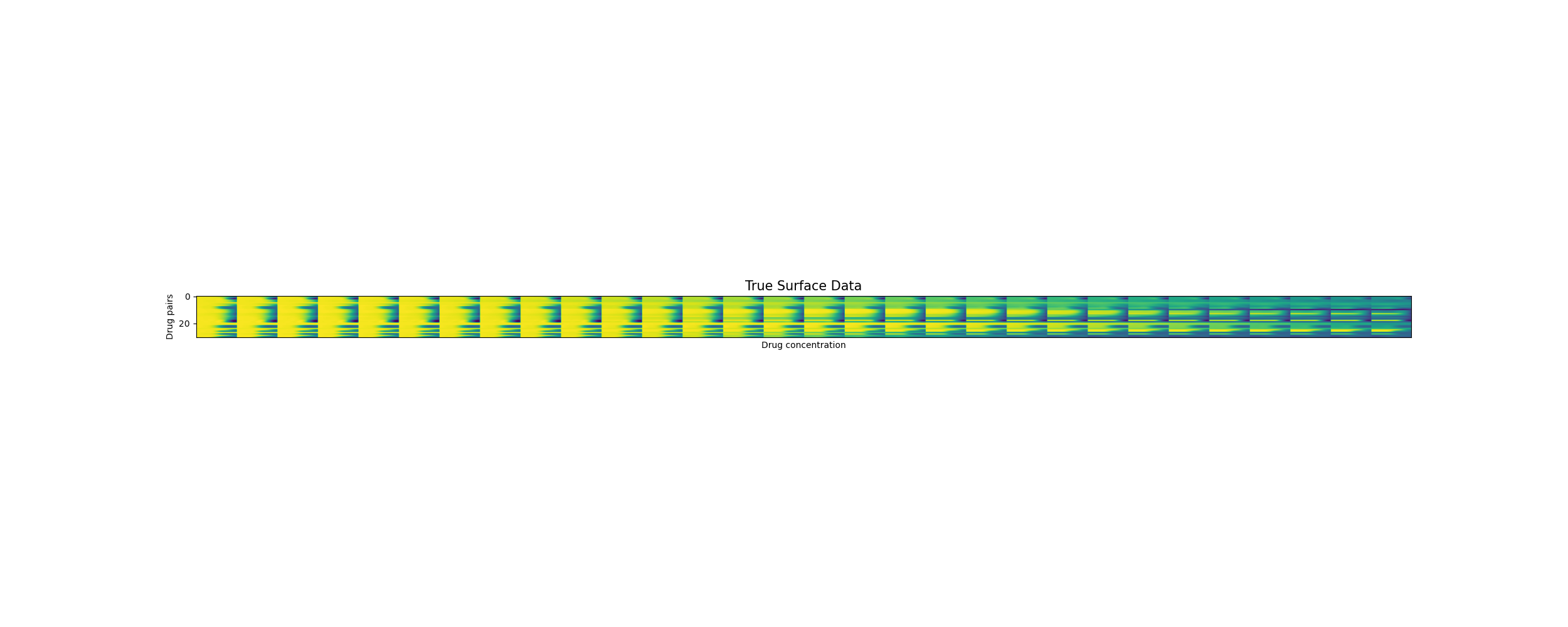
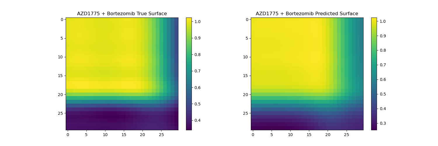
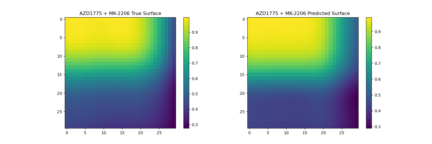
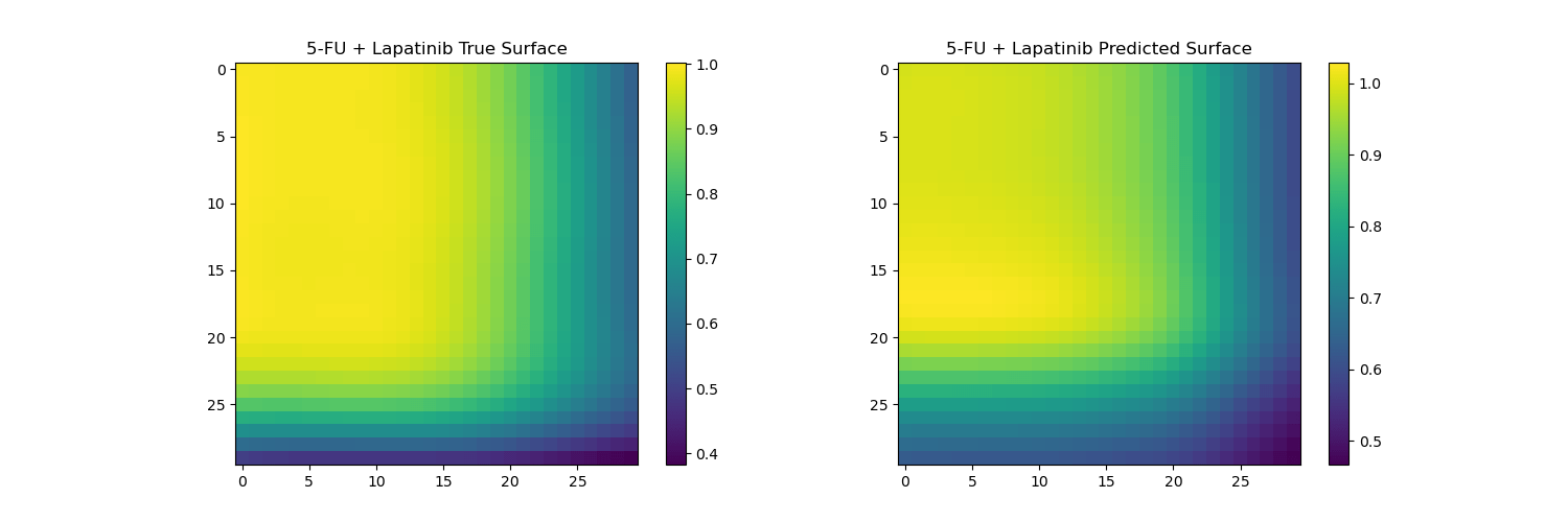
Predicting unseen drug surfaces (Y vs. $\hat{Y}$)

Drug pairs

Drug concentrations

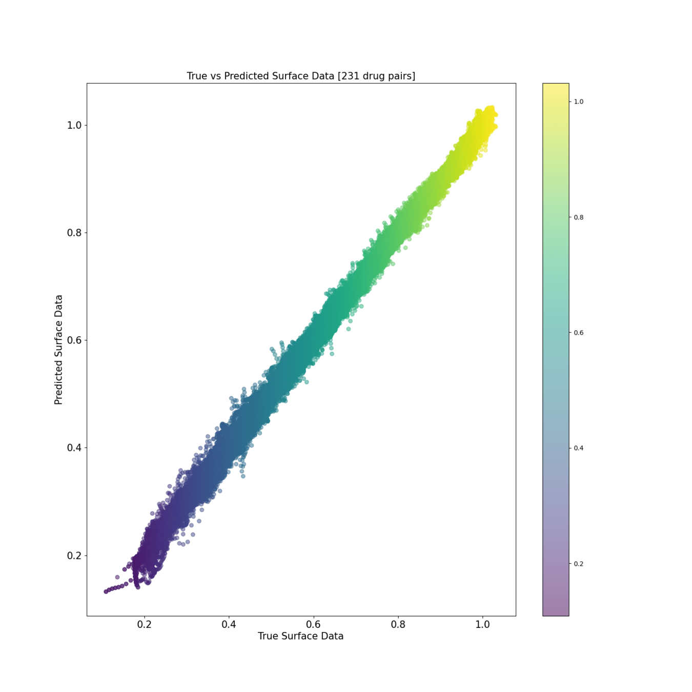
Training reconstruction [200 drug pairs]

Flattened drug surfaces

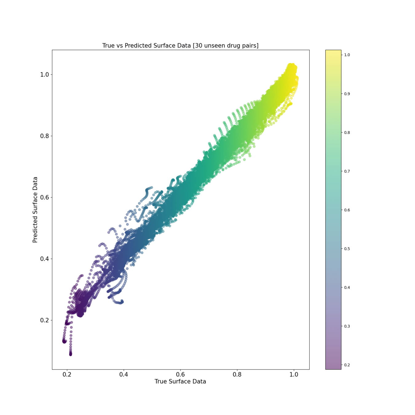
Test reconstruction [30 unseen pairs]

Scatter view of predicted drug synergies: Training and Test

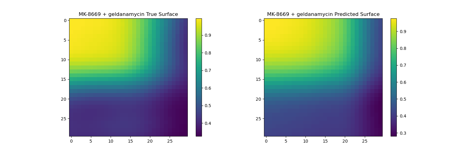
Surface reconstruction from coefficients on unseen drugs

Surface reconstruction from coefficients on unseen drugs

The predicted surfaces are good at capturing the overall shape of the surface but their variations are smoother than the real viabilities.

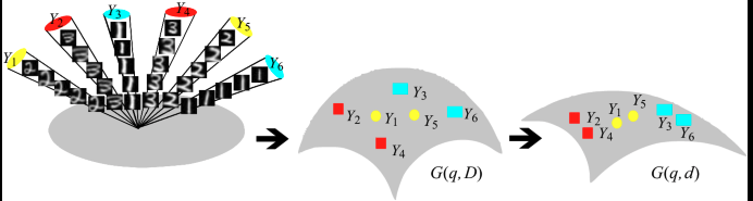
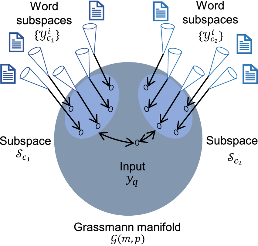
Extensions: Geometry view

Thank you!

What about generalising to unseen cell-lines (harder than for drugs, more variation)?

When you run SVD, you are selecting a point on the Grassmann manifold,

$D),\mathrm{Gr}(K,\,D),$

the set of all $K$ -dimensional linear subspaces of a $D$ -dimensional ambient space (D = G x G).

So the PCA subspace is a single point $[U*]$ on Gr(K,D) $[U⋆][U_\star$ $Gr(K,D)\mathrm{Gr}(Gr(K,D)$

The space $Gr(K,D)\mathrm{Gr}(K,D)$ is not Euclidean; its elements are subspaces but what is useful about this view is that it gives a natural metric for comparing subspaces, distances between subspaces, interpolation and traversal.

If later you learn a new subspace $UnewU_\text{new}$ (say, from new data or another cell line), you can treat both as points on $Gr(K,D)\mathrm{Gr}(K,D)$ and study their alignment via principal angles, this tells you whether the shape manifold of responses has shifted.

CU Group Meeting 14/11

By Vidhi Lalchand

CU Group Meeting 14/11

Vidhi Lalchand

Postdoctoral Fellow, Broad and MIT

vidhilalchand.co.uk

Modelling Cancer Drug Synergy Surfaces with Gaussian Processes

Interpretation

CU Group Meeting 14/11

More from Vidhi Lalchand