Shenfun - automating the spectral Galerkin method
Associate Professor Mikael Mortensen
Department of Mathematics
Division of Mechanics
University of Oslo
MekIT'17, Trondheim 11/5 - 2017
Spectral methods
what? why? where?

- Global basis (test) functions
- Typically Chebyshev or Legendre polynomials or Fourier exponentials
- Simple tensor product grids
- Smooth solutions
u(x) = \displaystyle\sum_{k=0}^{N-1} \hat{u}_k \phi_k(x)
Solution
Expansion coefficients
(unknowns)
Test functions
Spectral methods
what? why? where?
- Accuracy!
- Efficiency! Fast Fourier transforms
- and they're cool
u(x) = \displaystyle\sum_{k=0}^{N-1} \hat{u}_k \phi_k(x)
Solution
Expansion coefficients
(unknowns)
Test functions
Why not? Only simple cartesian domains unless you do spectral elements
Spectral methods
what? why? where?

3D + time and HUGE resolution
Serious number crunching - extreme computing
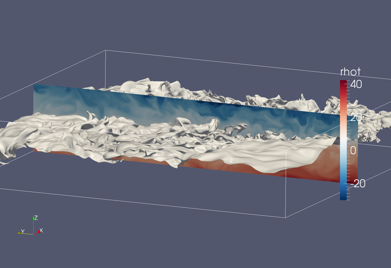
Images from huge spectral DNS simulations by S. de Bruyn Kops, UmassAmherst, College of Engineering
- Direct Numerical Simulations (DNS)
- Turbulent/transitional flows
- Instabilities/perturbations
- +++
DNS codes are usually written using low-level Fortran or C. Does it have to be this way?
Isn't it possible to do this just as well in a nice language like Python?
What does it really take to build a spectral DNS solver?
Numpy is designed around structured arrays that can be reshaped, resized, sliced, transposed, etc.
Most array operations are performed in C and are very fast

(1) Structured grid
(2) 3D parallel FFT

Numpy wraps FFTpack
pyFFTW wraps FFTW
No MPI
But mpi4py wraps almost the entire MPI library and is as efficient as low-level C

3D FFT with MPI
Slab decomposition (max N CPUs)
rfft2(a, axes=(0,1))
fft(a, axis=2)
Real space
Spectral space
4 processors - 4 colours
Do serial FFTs on local data
then transfer and realign datastructures
Do FFT in newly aligned direction
MPI.Alltoall
With now publicly available packages in
mpiFFT4py
mpi4py-fft
https://bitbucket.org/mpi4py/mpi4py-fft
With Licandro Dalcin at KAUST
Completely generic implementation - 500 lines of Python code
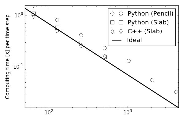
Both scaling very well on
thousands of CPUs
With parallel 3D FFT we may develop DNS solvers
Enstrophy colored by pressure
which turns out to be very easy, and
100 lines of compact Python code is enough to implement

Approximately 30% slower than C
Easily optimized the last 30% using Cython
Using just Fourier
Navier-Stokes is easy, what about other PDEs? non-periodic BCs?
\phi_k(x) = T_k(x)-T_{k+2}(x)
\phi_k(x) = L_k(x) - L_{k+2}(x)
Chebyshev
Legendre
(1) Choose spectral basis functions satisfying boundary conditions, e.g.:
\phi_k(\pm 1) = 0
(2) Transform PDEs using the method of weighted residuals -> variational forms
Best answer: The Spectral Galerkin method
Sounds easy? - Let's automate!
shenfun
from fenics import *

mesh = UnitSquareMesh(8, 8)
V = FunctionSpace(mesh, 'CG', 1)

# Define variational problem
u = TrialFunction(V)
v = TestFunction(V)
f = Constant(-6.0)
a = inner(grad(u), grad(v))*dx
L = f*v*dx
Solve equations with code very similar to mathematics
However
- Finite accuracy (not spectral)
- Not optimal for simple tensor product grids or DNS
How to automate?
What do we know about
automating the solution
of PDE'S?
Shenfun
Python package for automating the spectral Galerkin method
for high performance computing on tensor product grids
A FEniCS like interface with a simple form language
Extremely fast solvers for Poisson, Helmholtz and Biharmonic problems
MPI - invisible to the user
Fourier - Chebyshev - Legendre
modified basis functions
What else is there?
Chebfun
Spectral collocation, MATLAB, structured, no MPI
Semtex
Spectral element, MPI, C++/Fortran, 2D unstructured (1 Fourier)
Quite low-level, nowhere near as easily configured as FEniCS for new types of equations.
Very good for Navier-Stokes
Nek5000
Spectral element, Fortran, MPI, 3D unstructured
Nektar++
Spectral hp-element, C++, 3D unstructured
Nothing really for fast development of new spectral solvers aimed at high performance computing on supercomputers
Spectral Galerkin
Poisson example
\nabla^2 u(x) = f(x) \quad \text{for} \quad x \in [-1, 1]
u(\pm 1) = 0
Create a basis that satisfies boundary conditions, e.g.,
\phi_k(x) = T_k(x) - T_{k+2}(x) \quad V = \text{span}\{\phi_k\}_{k=0}^{N-3}
\displaystyle \int_{-1}^{1}v \nabla^2 u \, w dx = \int_{-1}^{1} vf w dx \quad \text{for all} \, v \in V
\text{Find } u \in V, \text{such that}
\text{where } w(x) \text{ is a weight function and } v \text{ is a test function}
Shenfun implementation
import numpy as np
from shenfun import TestFunction, TrialFunction, inner, div, grad, chebyshev

N = 20
V = chebyshev.ShenDirichletBasis(N, plan=True)
v = TestFunction(V)
u = TrialFunction(V)

# Assemble stiffness matrix
A = inner(v, div(grad(u)))

# Some consistent right hand side
f = Function(V, False)
f[:] = -2

# Assemble right hand side
f_hat = inner(v, f)

# Solve equations and transform spectral solution to real space
f_hat = A.solve(f_hat)
fj = V.backward(f_hat)

x = V.mesh(N)
assert np.allclose(fj, 1-x**2)
Very similar to FEniCS!
just with spectral accuracy
(1) Create basis
(2) Variational forms
2D/3D Tensor product spaces
Combinations of Fourier and Chebyshev/Legendre bases
u(x,y,z,t) = \displaystyle \sum_{k}\sum_{l}\sum_{m} \hat{u}_{k,l,m}(t) \phi_k(x)\phi_l(y)\phi_m(z)
W(x,y,z) = V(x) \times V(y) \times V(z)
Any combination of spaces (ultimately)
With solutions of the form:
Unknown expansion coefficients
2D/3D Tensor product spaces
Combinations of Fourier and Chebyshev/Legendre bases
from shenfun import *
from mpi4py import MPI

comm = MPI.COMM_WORLD
N = (20, 30)
V0 = chebyshev.ShenDirichletBasis(N[0])
V1 = fourier.R2CBasis(N[1])
T = TensorProductSpace(comm, (V0, V1))
v = TestFunction(T)
u = TrialFunction(T)

A = inner(v, div(grad(u)))

# Or 3D
V2 = fourier.C2CBasis(40)
T3 = TensorProductSpace(comm, (V0, V2, V1))
v = TestFunction(T3)
u = TrialFunction(T3)

A = inner(v, div(grad(u)))
MPI under the hood
using mpi4py-fft
on tensor product grids like:
A simple form language
to make implementation very similar to mathematics
Mathamatical operators act on test, trial, or functions with data
V = TensorProductSpace(comm, (V0, V1, V2))

# Form arguments:
v = TestFunction(V)
u = TrialFunction(V)
u_ = Function(V, False)

# Forms
du = grad(u_)
d2u = div(du)
cu = curl(du)
dudx = Dx(u_, 0)
Inner products and projections
A = inner(v, u)    # Bilinear form, assembles to matrices
f = inner(v, u_)   # Linear form, assembles to vector
project(div(grad(u_)), V)  # projection to V
Fast transforms
(not in FEniCS)
u_ = V.backward(u_hat, u_)Any spectral function is defined as
u(x) = \displaystyle\sum_{k=0}^{N-1} \hat{u}_k \phi_k(x)
u(x,y,z) = \displaystyle\sum_{k=0}^{N-1} \sum_{l=0}^{N-1} \sum_{m=0}^{N-1} \hat{u}_{klm} \phi_k(x)\phi_l(y)\phi_m(z)
3D:
1D:
This is computed on the tensor product grid as a backwards transform,
e.g., a discrete Fast Fourier inverse transform
A non-periodic basis uses fast Chebyshev transforms
Fast forward transforms
by L2-projections
u_hat = V.forward(u_, u_hat)(u_h, v_h) = (Iu, v_h)\quad \forall \, v_h \in V_h
\text{Find } u_h \in V_h, \text{such that}
which is achieved using a forward transform
Implemented with FFTs or fast Chebyshev transforms
Vector spaces
VectorTensorProductSpace
import numpy as np
from shenfun import *

N = 16
K0 = C2CBasis(N)
K1 = C2CBasis(N)
K2 = R2CBasis(N)
T = TensorProductSpace(comm, (K0, K1, K2))

# Scalar function u_
u_ = Function(T, False)
u_hat = Function(T)
u_[:] = np.random.random(u_.shape)
u_hat = T.forward(u_, u_hat)

# Now define vector space to allow computation of grad(u_)
TV = VectorTensorProductSpace([T]*3)
du_hat = project(grad(u_), TV, uh_hat=u_hat)
Nonlinearities
are all treated with pseudospectral techniques
\nabla u \times \nabla \times u
u \cdot u
u | u |^2
(1) Compute inverse
u = T.backward(u_hat)with dealiasing using
3/2-rule (padding) or 2/3-rule
(3) Transform back to spectral space
w = u*u(2) Compute nonlinearity
w_hat = T.forward(w)T = TensorProductSpace(comm, (V0, V1, V2))Complex Ginzburg-Landau
example
\frac{\partial u}{\partial t} = \nabla^2 u + u -(1+1.5i)u |u|^2
2D periodic (x, y) \( \in [-50, 50]^2 \)
Use Fourier in both directions
Weak form, only spatial discretization
\frac{\partial (v, u)^N}{\partial t} = -(\nabla v, \nabla u)^N + (v, u -(1+1.5i)u |u|^2)^N
(2\pi)^2\frac{\partial \hat{u}}{\partial t} = -(\nabla v, \nabla u)^N + (v, u -(1+1.5i)u |u|^2)^N
Complex Ginzburg-Landau
example
\frac{\partial u}{\partial t} = \nabla^2 u + u -(1+1.5i)u |u|^2
2D periodic (x, y) \( \in [-50, 50]^2 \)
import sympy
from shenfun.fourier.bases import R2CBasis, C2CBasis
from shenfun import inner, grad, TestFunction, TrialFunction, Function, \
    TensorProductSpace

# Use sympy to set up initial condition
x, y = sympy.symbols("x,y")
ue = (x + y)*sympy.exp(-0.03*(x**2+y**2))

N = (200, 200)
K0 = C2CBasis(N[0], domain=(-50., 50.))
K1 = C2CBasis(N[1], domain=(-50., 50.))
T = TensorProductSpace(comm, (K0, K1))
u = TrialFunction(T)
v = TestFunction(T)

def compute_rhs(rhs, u_hat, U, Up, T, Tp, w0):
    rhs.fill(0)
    rhs = inner(grad(v), -grad(U), output_array=rhs, uh_hat=u_hat)
    rhs /= (2*np.pi)**2
    rhs += u_hat
    rhs -= T.forward((1+1.5j)*U*abs(U)**2, w0)
    return rhs

# And, e.g., Runge-Kutta integrator
#
#
Key code:
Navier Stokes
Turbulent channel flow
3D tensor product space
2 Fourier bases +
Modified Chebyshev bases for wall normal direction
Kim and Moin modified version of Navier-Stokes:
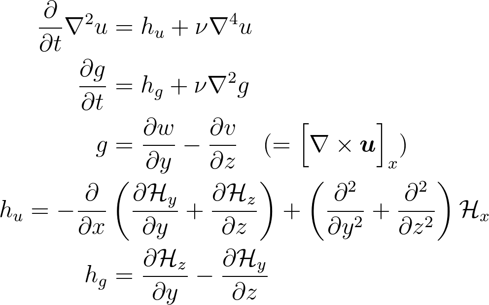
\mathcal{H}
is convection
Wall normal velocity
Wall normal vorticity
Navier Stokes
Turbulent channel flow
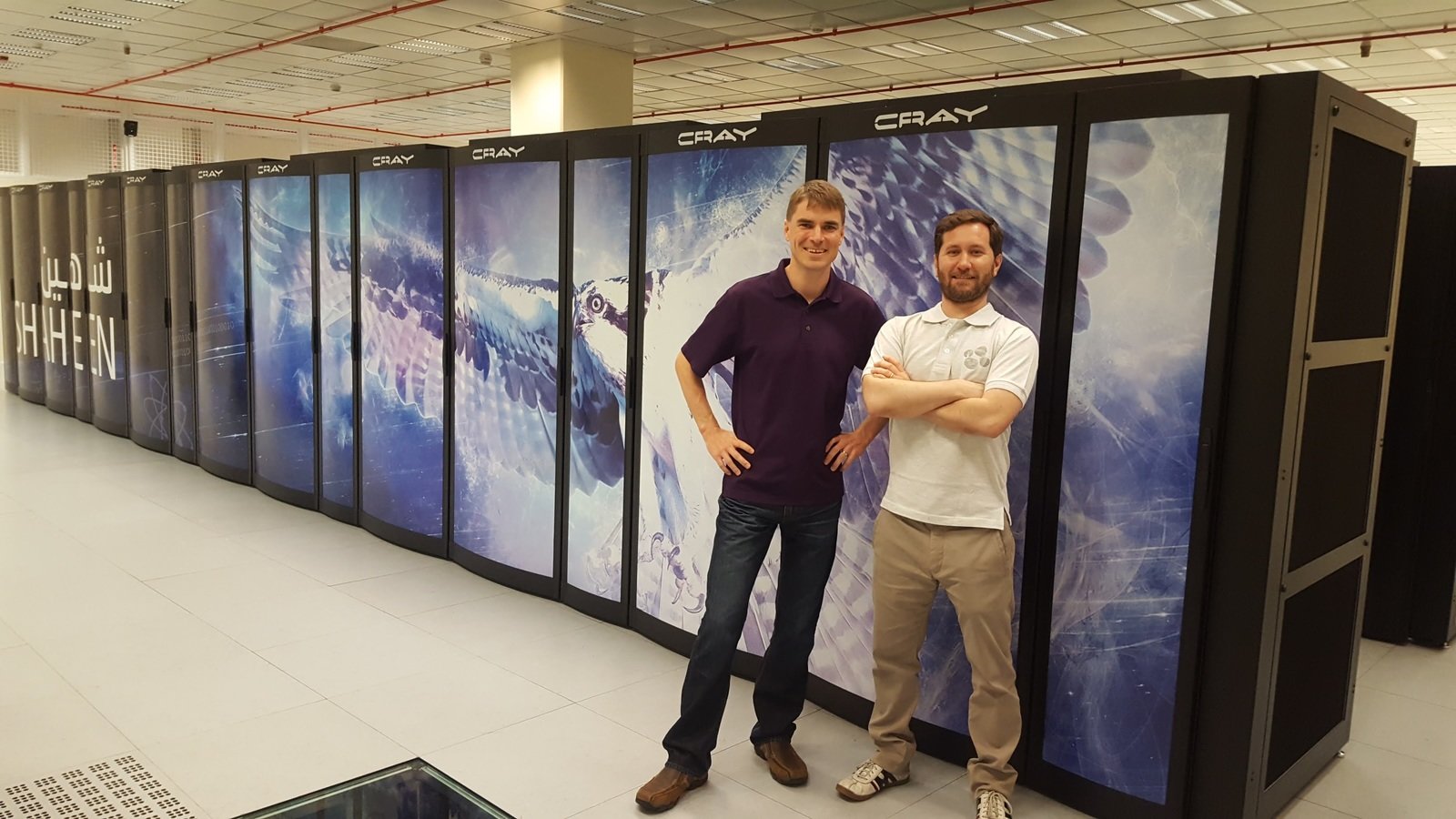
512\times 1024\times 1024
1 sec per time step on 512 cores
Tensor product mesh:
Shaheen II at KAUST
Thank you for your time! Questions?
http://github.com/spectralDNS

Presented at MekIT'17, Trondheim 11/5-2017
By Mikael Mortensen


