The SpectralDNS project:
Shenfun - automating the spectral Galerkin method
Associate Professor Mikael Mortensen
Department of Mathematics, Division of Mechanics, University of Oslo
I3MS-seminar RWTH Aachen University 6/11 - 2017

Outline of talk
Python for high performance scientific computing

Shenfun
A software for automating the spectral Galerkin method
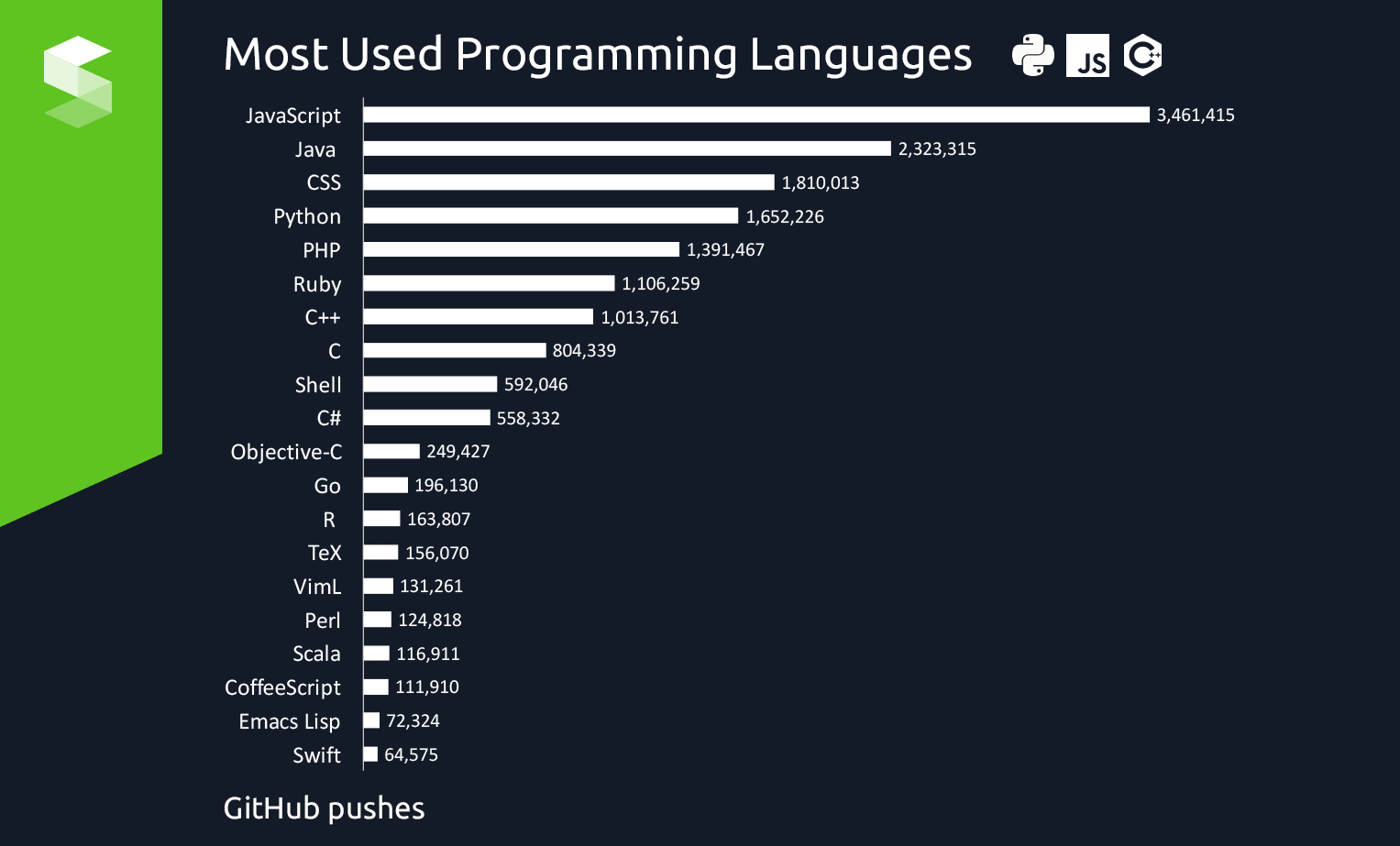
Github pushes by language (2017):
- An extremely usable, high-level programming language
- Very popular in the scientific computing community
- Open source
- Interpreted "scripting" language (no compilation)

Python vs Matlab
Python is often compared to Matlab, because a lot of the coding done in either is similar
- Python is a programming language, whereas Matlab is a numerical computing environment. Numpy+Scipy+Matplotlib is a numerical computing environment in Python.
- Python is open source and free, whereas Matlab is very expensive.
- Both have strong support for array manipulations and vectorization/slicing of arrays.
- Both are interpreted scripting languages. No compilation
- Python is easy to extend with MPI - Matlab is not
| Matlab | Python/Numpy | Operation |
|---|---|---|
| find(a>0.5) | nonzero(a>0.5) | find the indices where (a > 0.5) |
| zeros((3,4,5)) | zeros(3,4,5) | Create array of shape (3,4,5) |
| eye(3) | eye(3) | 3x3 identity matrix |
Some similarities and differences:
Anaconda Python
If you want to get started with scientific computing in Python

Comes pre-loaded with (almost) everything needed to do scientific computing
- Numpy - for array manipulations
- Scipy - Scientific library
- Matplotlib - for plotting
- mpi4py - Wraps MPI
- scikit-learn - machine learning and data mining
- +++
More than 1,500,000 downloads
https://anaconda.org

Using Fourier transformed Navier Stokes equations
Direct Numerical Simulations (DNS) of turbulence are traditionally performed with low-level Fortran or C
8192^3 \text{ mesh}
Part I: Python in high performance computing
Would it be possible to write a competitive, state of the art turbulence solver in Python?
From scratch?
(Not just wrapping a Fortran solver)
Using only standard Python modules numpy/scipy/mpi4py?
Can this solver be made to run on thousands of cores ?
With billions of unknowns?
As fast as C/fortran?
What does it take to build a spectral DNS solver?


Triply periodic domain
Fourier space
[0, 2 \pi]^3
Equations:
What does it take to build a spectral DNS solver?

Navier Stokes in spectral (Fourier) space:
Pseudo-spectral treatment of nonlinearity
Some timestepping routine (e.g., 4th order Runge-Kutta)
Classical pseudo-spectral Navier-Stokes solver
The kind that has been used to break records since the day of the first supercomputer
What does it really take to implement a spectral DNS solver?
Numpy is designed around structured arrays that can be reshaped, resized, sliced, transposed, etc.
Most array operations are performed in C and are very fast

(1) Structured grid
(2) 3D parallel FFT

Numpy wraps FFTpack
pyFFTW wraps FFTW
MPI ?
But MPI for Python ( mpi4py, Lisandro Dalcin) wraps almost the entire MPI library and is as efficient as low-level C

Implementation
A few computational details
A computational box (mesh) needs to be distributed between a large (possibly thousands) number of processors
N^3, N \sim 1000 - 10000
Mesh size:
Pencil
Slab
\le N^2
CPUs
\le N
CPUs
3D FFT with MPI
in a nutshell
real FFT in z, complex in y
No MPI required
Transpose and distribute
Then FFT in last direction
- 2D FFTs in Y-Z planes (local)
- transpose operation
- distribute data (MPI Alltoall)
- FFT in X-direction
What does it really take?
4 operations, four lines of Python code!
Pencil decomposition
in a nutshell
rfft(u, axis=2)
Transform
fft(u, axis=0)
Transform
fft(u, axis=1)
7 operations
-
FFT z-dir
-
transpose
-
communicate
-
FFT y-dir
-
transpose
-
communicate
-
FFT x-dir
7 lines of code!
With parallel 3D FFT we may develop parallel DNS solvers
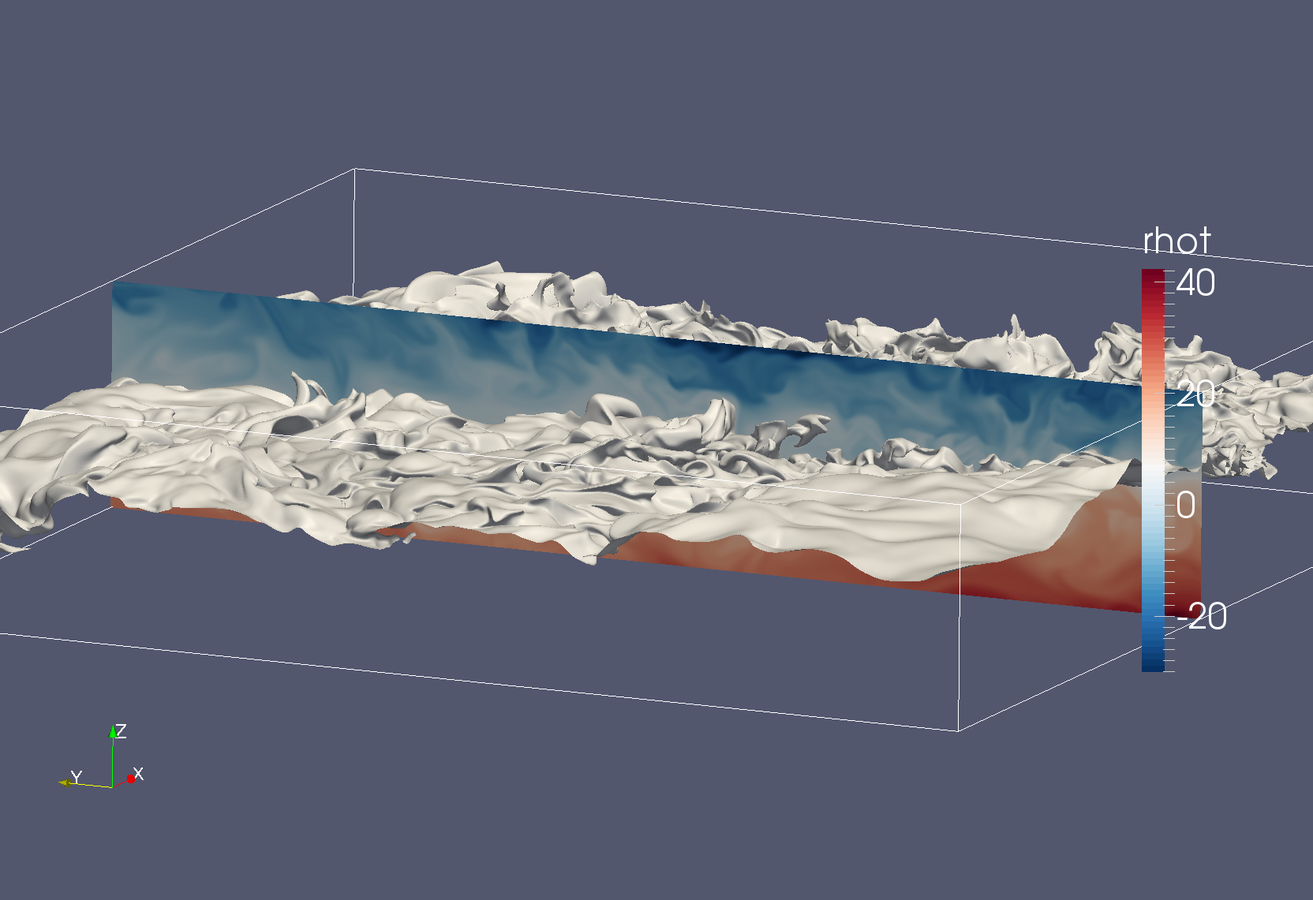
Enstrophy colored by pressure
and
100 lines of compact Python code is enough to implement
Ok, so it was relatively easy to implement
How about speed and parallel scaling?
Can we compete with low-level C/C++ or Fortran on supercomputers?
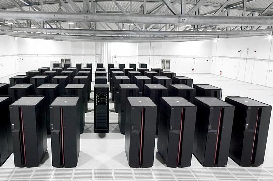
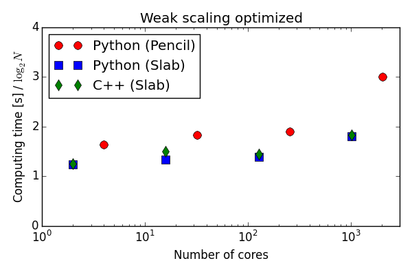
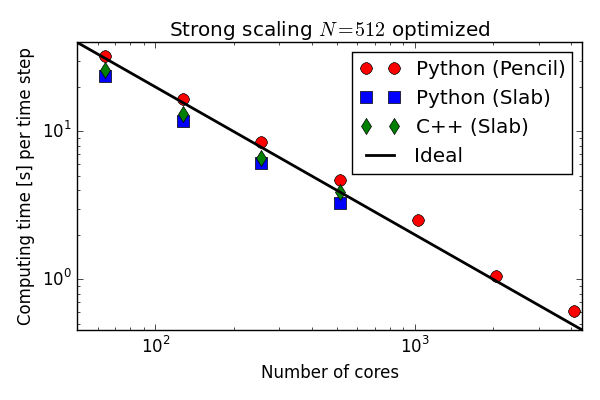
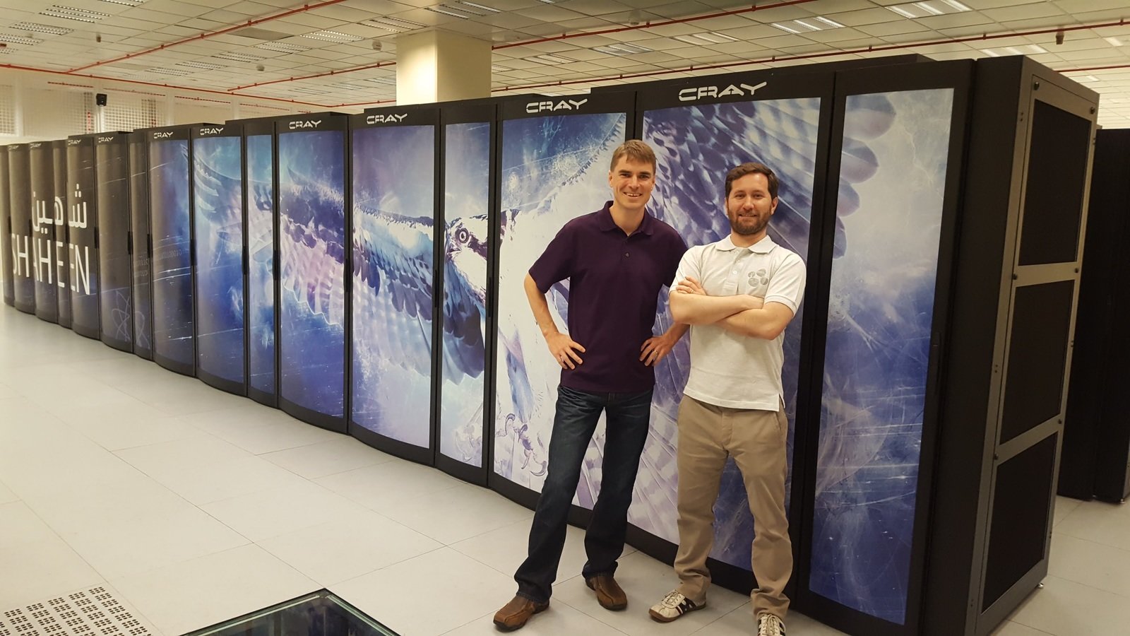
Parallell scaling
Shaheen Blue Gene P supercomputer at KAUST Supercomputing Laboratory
Testing the 100 lines of pure Python code in parallel
C++(slab) 20-30 % faster than Python (slab)
Good strong scaling
mesh =
2048^3
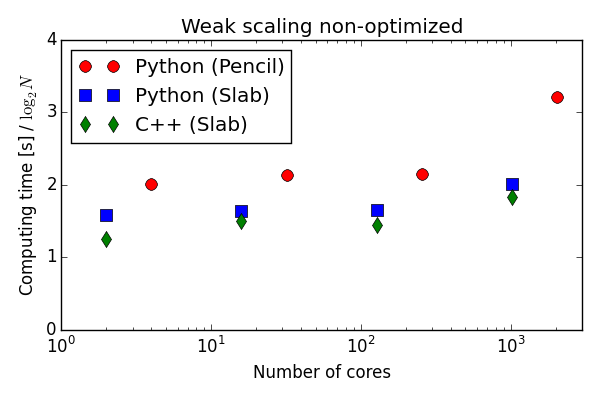
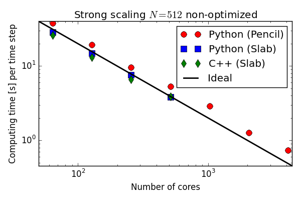
512^3
Why slower than C++?
Actually, the numpy ufuncs used to compute the cross product is the main reason
Luckily Python has several options for optimizing slow code
Moving cross product to Cython or Numba
def cross(a, b, c):
    c[0] = a[1]*b[2]-a[2]*b[1]
    c[1] = a[2]*b[0]-a[0]*b[2]
    c[2] = a[0]*b[1]-a[1]*b[0]
    return c

u = np.ones((3, N, N, N))
w = np.ones((3, N, N, N))
v = np.zeros((3, N, N, N))
v = cross(u, w, v)
Numpy has to create intermediate work arrays on the fly
Hardcoding the cross product into one single loop
@jit(float[:,:,:,:](float[:,:,:,:], float[:,:,:,:], float[:,:,:,:]), nopython=True)
def cross(a, b, c):
    for i in xrange(a.shape[1]):
        for j in xrange(a.shape[2]):
            for k in xrange(a.shape[3]):
                a0 = a[0,i,j,k]
                a1 = a[1,i,j,k]
                a2 = a[2,i,j,k]
                b0 = b[0,i,j,k]
                b1 = b[1,i,j,k]
                b2 = b[2,i,j,k]
                c[0,i,j,k] = a1*b2 - a2*b1
                c[1,i,j,k] = a2*b0 - a0*b2
                c[2,i,j,k] = a0*b1 - a1*b0
    return c
Either Cython or Numba will do the trick. A few lines more
Numba and Cython perform approximately the same
and as fast as C++!
Approximately 5 times faster than original
Solver optimized with Cython
More than matches C++ on the Blue Gene P!
On an even larger supercomputer
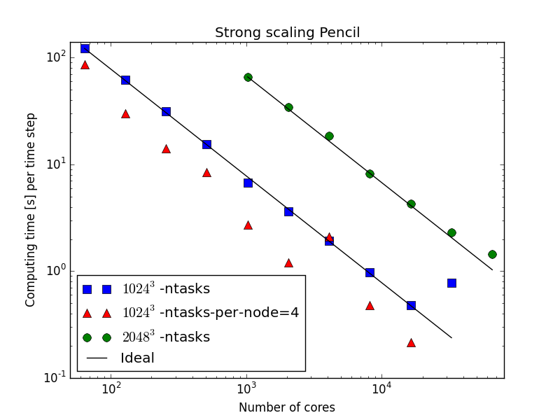
64^3
mesh size = per task
65536 tasks!
mesh =
per task
Word of warning
2048 nodes, or 65536 tasks, take about 13 minutes to load Python and get started
0.5 \cdot 64^3
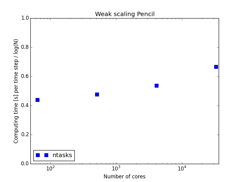
Concept proven
Python can be used for high performance supercomputing and it can be used for DNS with Fourier
mpi4py-fft
https://bitbucket.org/mpi4py/mpi4py-fft
With Lisandro Dalcin at KAUST
~ 500 lines of Python code
With the newly released
we can do any transform from FFTW in parallel
Highly configurable and fast
Part II of talk
Automating the spectral Galerkin method
on non-periodic domains, with different types
of boundary conditions (Dirichlet/Neumann)
Not just periodic Fourier
With a highly configurable library for any fast transforms
we can now implement the spectral Galerkin method
The spectral Galerkin method
Galerkin meets orthogonal
global spectral basis functions, e.g.
- Chebyshev
- Legendre
- Fourier
\left( u, v \right)_w = \int_{\Omega} u\, v^* \, w\, dx
u(x) = \displaystyle\sum_{k=0}^{N-1} \hat{u}_k \phi_k(x)
Solution
Expansion coefficients
(unknowns)
Global basis functions
We use it to solve PDEs using the method of weighted residuals
Weighted inner products:
The spectral Galerkin method
works in three steps
-
Choose global basis (test) functions satisfying the correct boundary conditions. Usually modified Chebyshev or Legendre polynomials, or Fourier exponentials
-
Transform PDEs to weak variational forms using the method of weighted residuals
-
Assemble and solve linear system of equations
Spectral Galerkin
Poisson example
\nabla^2 u(x) = f(x) \quad \text{for} \quad x \in [-1, 1]
u(\pm 1) = 0
1) Create a basis that satisfies boundary conditions, e.g.,
\phi_k(x) = L_k(x) - L_{k+2}(x) \quad V = \text{span}\{\phi_k\}_{k=0}^{N-3}
\displaystyle \int_{-1}^{1}v \nabla^2 u \, w dx = \int_{-1}^{1} vf w dx
\text{where } w(x) \text{ is a weight function and } u \in V \text{ is trial function}
(Legendre polynomial order k+2)
2) Transform PDE to variational form using test function
v \in V
3) Assemble and solve linear system of equations
\text{Find } u \in V, \text{such that}
\left(v, \nabla^2 u \right)_w^N = \left(v, f \right)_w^N \quad \forall v \in V
\left( v, u\right)_w^N \approx \displaystyle \int_{-1}^{1} vu^* w dx
u(x) = \displaystyle\sum_{j=0}^{N-1} \hat{u}_j \phi_j(x)
v(x) = \phi_k(x)
Trial function
Test function
With quadrature notation
\left( \phi_k, \sum_j \hat{u}_j \phi_j^{''} \right)_w^N = \left( \phi_k, f\right)_w^N
A_{kj} \hat{u}_j = \tilde{f}_k
Insert to get linear algebra problem:
A_{kj} = \left( \phi_k, \phi_j^{''} \right)_w^N
With
3 steps - Sounds generic and easy?
Let's automate!
from fenics import *

mesh = UnitSquareMesh(8, 8)
V = FunctionSpace(mesh, 'CG', 1)

# Define variational problem
u = TrialFunction(V)
v = TestFunction(V)
f = Constant(-6.0)
a = inner(grad(u), grad(v))*dx
L = f*v*dx- Automates the finite element method (Galerkin)
- Code very similar to mathematics
- Basis functions with local support
-
Finite accuracy (not spectral)
How?
\int_{\Omega} \nabla u \cdot \nabla v dx
Shenfun
https://github.com/spectralDNS/shenfun
Python package (~3k loc) for automating the spectral Galerkin
method for high performance computing on tensor product grids
- A FEniCS like interface with a simple form language
- MPI - invisible to the user: mpi4py-fft
- Fourier - Chebyshev - Legendre modified basis functions
- Extremely fast (!), order optimal, direct solvers for Poisson, Helmholtz and Biharmonic problems

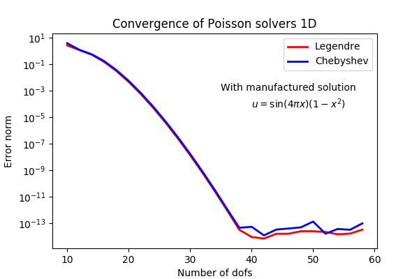
Shenfun implementation of 1D Poisson problem
import numpy as np
from shenfun import TestFunction, TrialFunction, inner, div, grad, chebyshev

N = 20
V = chebyshev.ShenDirichletBasis(N, plan=True)
v = TestFunction(V)
u = TrialFunction(V)

# Assemble stiffness matrix
A = inner(v, div(grad(u)))

# Some consistent right hand side
f = Function(V, False)
f[:] = -2

# Assemble right hand side
f_hat = inner(v, f)

# Solve equations and transform spectral solution to real space
f_hat = A.solve(f_hat)
fj = V.backward(f_hat)

x = V.mesh(N)
assert np.allclose(fj, 1-x**2)
Very similar to FEniCS!
just with spectral accuracy
(1) Create basis
(2) Variational forms
(3) Solve system
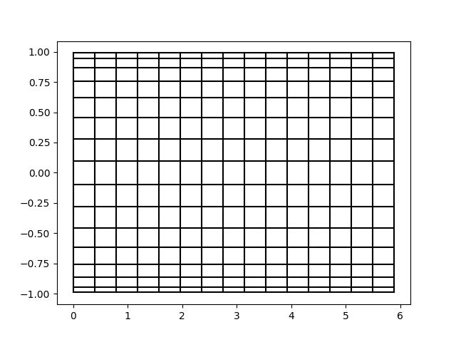
2D/3D/4D.. Tensor product spaces
Cartesian products of Fourier and Chebyshev/Legendre bases
u(x,y,z,t) = \displaystyle \sum_{k}\sum_{l}\sum_{m} \hat{u}_{klm}(t) \phi_k(x)\phi_l(y)\phi_m(z)
W(x,y,z) = V(x) \times V(y) \times V(z)
Any Cartesian combination of spaces (ultimately)
With solutions of the form:
Unknown expansion coefficients
Tensor product spaces
Implementation
from shenfun import *
from mpi4py import MPI

comm = MPI.COMM_WORLD
N = (20, 30)

# Create two bases
V0 = chebyshev.ShenDirichletBasis(N[0])
V1 = fourier.R2CBasis(N[1])

# Create tensor product space
T = TensorProductSpace(comm, (V0, V1))
v = TestFunction(T)
u = TrialFunction(T)

A = inner(v, div(grad(u)))

# Or 3D
V2 = fourier.C2CBasis(40)
T3 = TensorProductSpace(comm, (V0, V2, V1))
v = TestFunction(T3)
u = TrialFunction(T3)

A = inner(v, div(grad(u)))
MPI under the hood
using mpi4py-fft
on tensor product grids like:
Slab
Pencil
A simple form language
influenced heavily by UFL/FEniCS
Mathematical operators act on test, trial, or functions with data
V = TensorProductSpace(comm, (V0, V1, V2))

# Form arguments:
v = TestFunction(V)
u = TrialFunction(V)
u_ = Function(V, False)

# Forms
du = grad(u_)
d2u = div(du)
cu = curl(du)
dudx = Dx(u_, 0)
Inner products and projections
A = inner(v, u)    # Bilinear form, assembles to matrices
f = inner(v, u_)   # Linear form, assembles to vector
project(div(grad(u_)), V)  # projection to V
Fast transforms
u_hat = V.forward(u, u_hat) u = V.backward(u_hat, u)Move back and forth between and using fast transforms
Periodic basis using fast Fourier transforms
Non-periodic basis using fast Chebyshev transforms (not for Legendre)
\blue{u}
\blue{\hat{u}}
\blue{u}(x,y,z) = \displaystyle\sum_{k=0}^{N-1} \sum_{l=0}^{N-1} \sum_{m=0}^{N-1} \blue{\hat{u}_{klm}} \phi_k(x)\phi_l(y)\phi_m(z)
Nonlinearities
all treated with pseudo-spectral techniques
u \times \nabla \times u
u \cdot u
u | u |^2
(1) Compute inverse
u = T.backward(u_hat)with dealiasing using
3/2-rule (padding) or 2/3-rule
(3) Transform back to spectral space
w = u*u(2) Compute nonlinearity
w_hat = T.forward(w)T = TensorProductSpace(comm, (V0, V1, V2))Fast direct solvers
1D: \text{Find } u \in V, \text{such that}
\left(v, \nabla^2 u \right)_w^N = \left(v, f \right)_w^N \quad \forall v \in V
A_{kl} \hat{u}_l = \tilde{f}_k
\text{Leading to a linear algebra problem:}
Fourier: A is diagonal
Modified Legendre: A is diagonal
Modified Chebyshev: A sparse - solved as tridiagonal matrix
Fast direct solvers
2 dimensions
\left(v, \nabla^2 u \right)_w^N = \left(v, f \right)_w^N \quad \forall v \in V^1\times V^2
\text{Find } u \in V^1\times V^2, \text{such that}
A_{km}^1 B^2_{nl}\hat{u}_{mn} + B^1_{km} A^2_{nl} \hat{u}_{mn} = \tilde{f}_{kl}
Matrix form:
A^1 \hat{u} B^2 + B^1 \hat{u} (A^{2})^T = \tilde{f}
Sparse matrices A (stiffness) and B (mass) are 1D matrices of basis (1/2)
Very fast direct solvers implemented in parallel using matrix decomposition method
Linear algebra:
2D Poisson
in more detail
\nabla^2 u(x) = f(x) \quad \text{for} \quad x \in [0, 2\pi] \times [-1, 1]
u(x, \pm 1) = 0 \quad u(2\pi, y) = u(0, y)
from shenfun import *
from mpi4py import MPI
comm = MPI.COMM_WORLD
N = (64, 64)
K1 = R2CBasis(N[0])
SD = chebyshev.bases.ShenDirichletBasis(N[1])
T = TensorProductSpace(comm, (K1, SD))
u = TrialFunction(T)
v = TestFunction(T)
2D Poisson
Assemble matrix
Trial function
Test function
\phi_l(x) = \exp(ilx)
\phi_m(y) = T_m(y) - T_{m+2}(y)
Combination of Chebyshev polynomials (or Legendre) that satisfies boundary conditions
Jie Shen's modified basis satisfies bcs and leads to very sparse matrices
u(x, y) = \displaystyle \sum_{k, j} \hat{u}_{kj} \phi_k(x) \phi_j(y)
v(x, y) = \phi_l(x) \phi_m(y)
2D Poisson
Assemble matrices
(-k^2 B_{mj}^D + A_{mj}^D)\hat{u}_{kj}\quad \forall \, k=0,1,\ldots, N-1
1D stiffness
1D mass
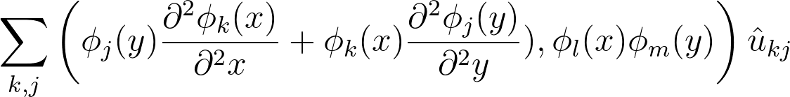
A_{lk}^{F} B_{mj}^{D}\hat{u}_{kj} + B_{lk}^{F} A_{mj}^{D} \hat{u}_{kj}
Matrix form
\text{Fourier matrices } B^F \text{ and } A^{F}
\text{ are diagonal }
\text{and can be eliminated, leaving N 1D problems:}
2D Poisson
Assemble matrices in shenfun
from shenfun import *
from mpi4py import MPI
comm = MPI.COMM_WORLD
N = (64, 64)
K1 = R2CBasis(N[0])
SD = chebyshev.bases.ShenDirichletBasis(N[1])
T = TensorProductSpace(comm, (K1, SD))
u = TrialFunction(T)
v = TestFunction(T)

mat = inner(div(grad(u)), v)
Creates mat - a dictionary holding two sparse matrices: mass and stiffness. Fourier contribution are scales to matrices
(-k^2 B_{mj} + A_{mj})\hat{u}_{kj}\quad \forall k=0,1,\ldots, N-1
Complex Ginzburg-Landau
example
\frac{\partial u}{\partial t} = \nabla^2 u + u -(1+1.5i)u |u|^2
2D periodic (x, y) \( \in [-50, 50]^2 \)
Use Fourier in both directions
Weak form, only spatial discretization:
\frac{\partial (v, u)^N}{\partial t} = -(\nabla v, \nabla u)^N + (v, u -(1+1.5i)u |u|^2)^N
(2\pi)^2\frac{\partial \hat{u}}{\partial t} = -(\nabla v, \nabla u)^N + (v, u -(1+1.5i)u |u|^2)^N
Complex Ginzburg-Landau
example
2D periodic (x, y) \( \in [-50, 50]^2 \)
import sympy
from shenfun.fourier.bases import R2CBasis, C2CBasis
from shenfun import inner, grad, TestFunction, TrialFunction, \
    Function, TensorProductSpace

# Use sympy to set up initial condition
x, y = sympy.symbols("x,y")
ue = (x + y)*sympy.exp(-0.03*(x**2+y**2))

N = (200, 200)
K0 = C2CBasis(N[0], domain=(-50., 50.))
K1 = C2CBasis(N[1], domain=(-50., 50.))
T = TensorProductSpace(comm, (K0, K1))
u = TrialFunction(T)
v = TestFunction(T)
U = Function(T, False)

def compute_rhs(rhs, u_hat, U, T):
    rhs = inner(grad(v), -grad(U), output_array=rhs, uh_hat=u_hat)
    rhs /= (2*np.pi)**2
    rhs += u_hat
    rhs -= T.forward((1+1.5j)*U*abs(U)**2, w0)
    return rhs

# And, e.g., Runge-Kutta integrator
#
#
Key code:
(2\pi)^2\frac{\partial \hat{u}}{\partial t} = -(\nabla v, \nabla u)^N + (v, u -(1+1.5i)u |u|^2)^N
Navier Stokes
Turbulent channel flow
3D tensor product space
2 Fourier bases +
Modified Chebyshev bases for wall normal direction
Kim and Moin modified version of Navier-Stokes:
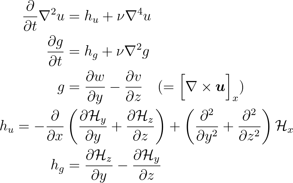
\mathcal{H}
is convection
Wall normal velocity
Wall normal vorticity
Navier Stokes
Turbulent channel flow
512\times 1024\times 1024
First fully spectral DNS with
3D Tensor product mesh:
Shaheen II at KAUST
\text{Re}_{\tau} > 2000
Some more demos
Thank you for your time!
http://github.com/spectralDNS/shenfun
Questions?
conda install -c conda-forge -c spectralDNS shenfun
Presented at I3MS-seminar Aachen 6/11-2017
By Mikael Mortensen


