
Computational Biology
(BIOSC 1540)
Jan 30, 2025
Lecture 04B
Gene prediction
Methodology
Announcements
Assignments
Quizzes
CBytes
ATP until the next reward: 1,783
After today, you should have a better understanding of
Problem formulation of gene prediction
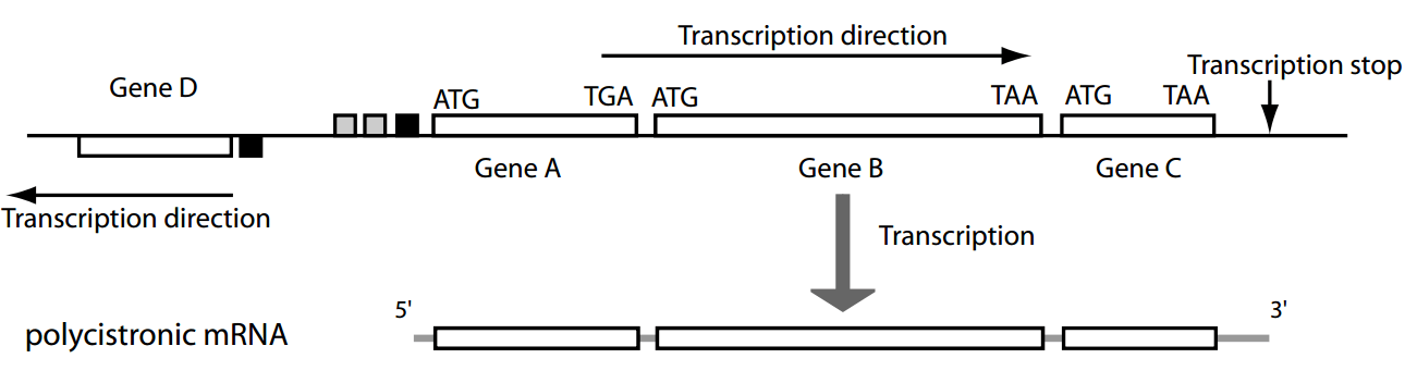
Gene prediction identifies protein-coding regions in a genome using computational methods
Gene prediction is essential for genome annotation and understanding gene function.
Predicted genes
DNA sequences contain a mix of coding and noncoding regions.
Early computational gene prediction methods detected genes by recognizing characteristic sequence patterns
However, reliance on fixed patterns limited accuracy in complex genomes
In the early days (1980s), gene prediction was based on hardcoded rules
Fickett, J. W. (1982). Recognition of protein coding regions in DNA sequences. Nucleic acids research, 10(17), 5303-5318.
- Codon position biases
- Start codons (e.g., ATG)
- Termination signals (e.g., TAA, TAG, TGA)
- Transcription start sites (e.g., TATA box)
For example, they would search for
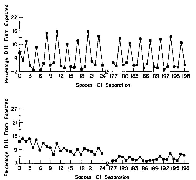
Autocorrelation of T in sequences
Coding
Non-coding
Relying on fixed patterns often leads to incorrect predictions
Many non-coding sequences contain patterns that mimic coding sequences, leading to high false positive rates
Not all genes follow the same start/stop codon rules, and promoter motifs are not always well-defined.
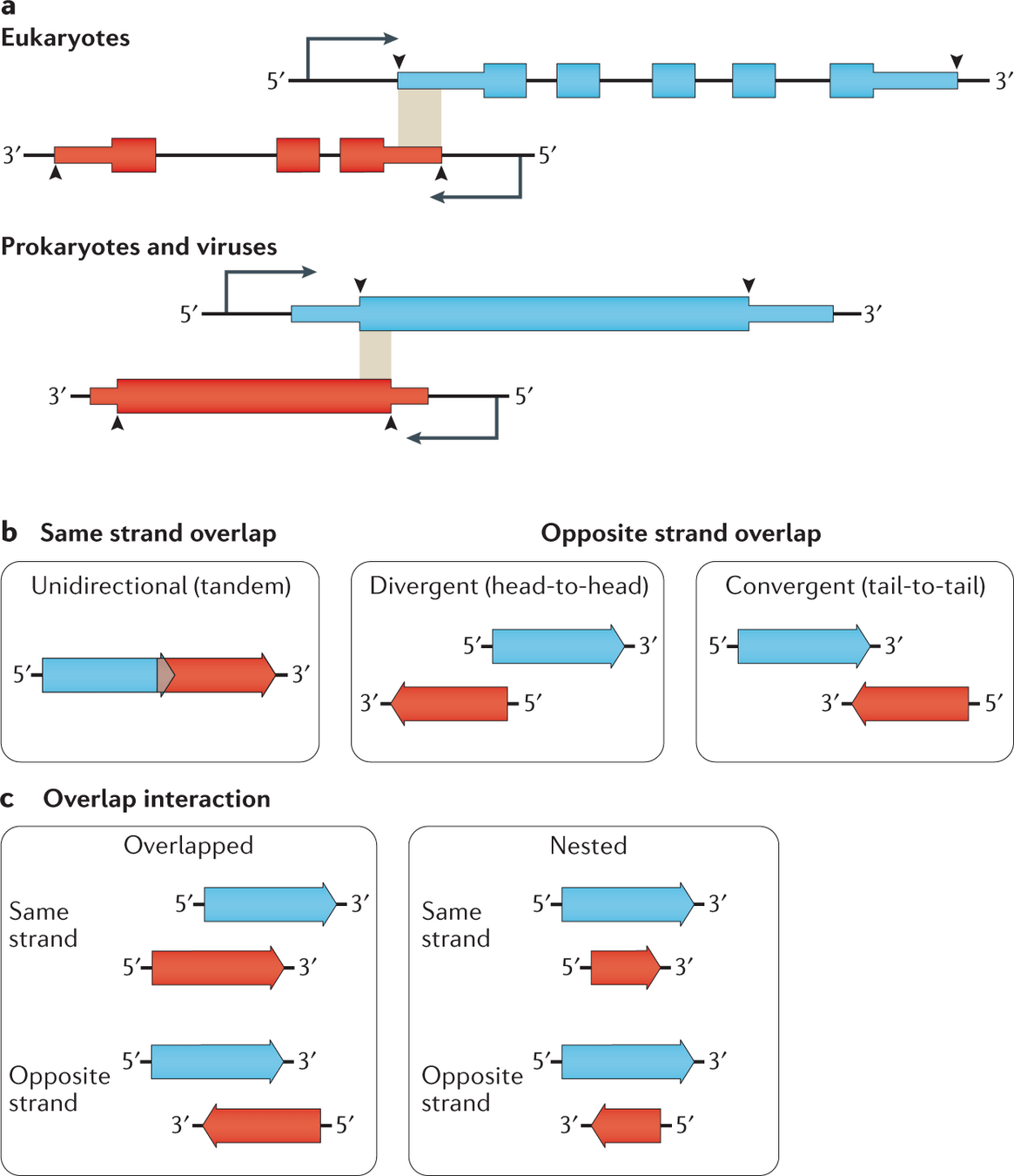
Some genes overlap or exist within other genes, making simple start/stop rules unreliable.
To improve accuracy, gene prediction must go beyond fixed patterns and incorporate statistical properties of real genes
After today, you should have a better understanding of
The fundamentals of probability and its role in modeling biological data
Conditional probability
Probabilistic Models Improve Gene Prediction
- Codon bias: Some codons appear more frequently in real genes.
- Sequence composition: GC content differences indicate coding regions.
-
Signal sequences: Start/stop codons, splice sites, and
promoter motifs have variable strengths.
Instead of using fixed rules, we use probabilistic models that quantify uncertainty
These models assign probabilities based on multiple features:
Some events occur independently, while others depend on previous observations
Gene prediction inherently relies on dependencies between nucleotides, codons, and genomic regions
Independent Events: The probability of one event does not affect another
Example: Rolling a die twice—each roll is unaffected by the previous one
Dependent Events: The probability of one event depends on another
Example: A sequence with a high GC-ratio is more likely to belong to a coding region.
Motivating example: Suppose we want to predict whether a sequence is a gene using its GC content
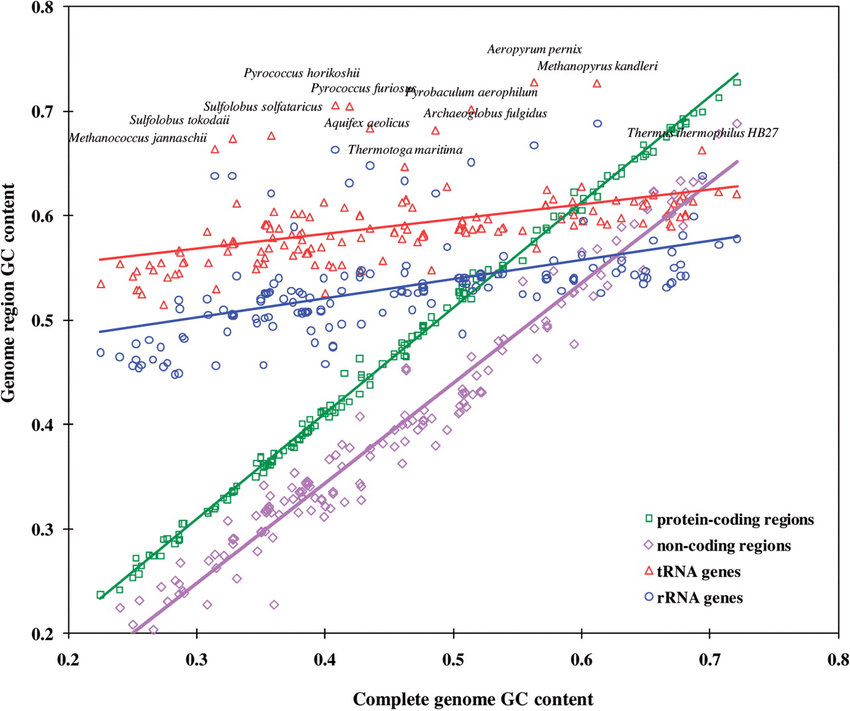
Genes often have higher GC content that surrounding non-coding regions
However, not all GC-rich regions are genes, and not all genes are GC-rich
Our goal is to update our belief (i.e., probability) about "gene-ness" based on a region's GC content
Joint probability is the statistical measurement of two events occurring at the same time
P ( \text{gene} \vert \text{GC-rich} )
P(\text{GC-rich})
Probability of being GC-rich
Probability that a region is a gene given that it's GC-rich
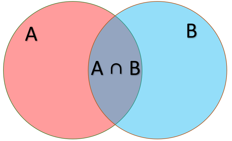
P(\text{gene} \cap \text{GC-rich})
Suppose I want to compute the probability of a region being both GC-rich and a gene
means "and" in set notation
\cap
P(\text{GC-rich}) P ( \text{gene} \vert \text{GC-rich} )
=
This is the (conditional) probability we want to know
Gene
GC-rich
Conditional probability allows us to refine dependent predictions based on new information
P ( \text{gene} \vert \text{GC-rich} ) = \frac{P(\text{gene} \cap \text{GC-rich})}{P(\text{GC-rich})}
Gene
GC-rich
Rearranging our equation allows us to compute the probability that a given region could be gene if it's GC-rich
If we have the following information available:
P(\text{gene} \cap \text{GC-rich})
P(\text{GC-rich})
Probability of a random region being a gene and GC-rich
Probability of a random region being GC-rich
We can compute these properties with known data
Challenge: Multiple signals can improve gene prediction
Why multiple signals?
- A single feature like GC-richness helps, but not all genes are GC-rich, and non-gene regions can be GC-rich too.
- Other signals include promoter motifs, codon bias, start/stop codons, etc.
Objective:
- Combine these signals to increase confidence in identifying gene regions.
- Challenge: How do we do this probabilistically without getting overwhelmed?
After today, you should have a better understanding of
The fundamentals of probability and its role in modeling biological data
Bayes' theorem
Using direct conditional probability for many signals requires enumerating multi-way intersections
P(\text{Gene} \mid X)
= \frac{P(\text{Gene} \cap X)}{P(X)}
Conditional probability for N signals,
For each new signal, you must compute a new, higher-dimensional intersection over the whole genome.
P(\text{Gene} \mid X_1, X_2, \dots, X_n) =
\frac{P(\text{Gene} \cap X_1 \cap X_2 \,\dots\, X_n)}{P(X_1 \cap X_2 \,\dots\, X_n)}
Conditional probability for one signal,
X
Enumerating multi-way intersections is cumbersome and lacks flexibility
Data Explosion:
- 2 features → 4-way sets (Gene vs. not-Gene, X1X_1X1 vs. not-X1X_1X1, etc.)
- 3 features → 8-way sets, and so on—this scales exponentially.
Changing Thresholds: If you redefine “GC-rich” from 60% to 65%, you have to recompute those entire intersections.
Interpretation Issues: Knowing the overlap doesn’t explain how each feature individually shifts the probability that we have a gene.
Bayes’ Theorem provides a more modular, flexible way to incorporate multiple signals
Conditional probability for N signals (and after some math)
P(\text{Gene} \mid X_1, \dots, X_n)
\;\propto\;
P(\text{Gene})\,\prod_{i=1}^{N} P(X_i \mid \text{Gene})
P(\text{Gene})
P(X_i \mid \text{Gene})
Measure
just once and separately measure
P(X_{N+1} \mid \text{Gene})
X_{N+1}
Adding a new signal
just requires
P(X_i \mid \text{Gene})
Each
shows how strongly feature
X_{i}
indicates a gene
Advantages
When you want to rank or compare classes based on posterior probability, you can ignore the denominator
Biological sequences also have inherent dependencies that require more than Bayes' formula
Bayes’ Theorem allows us to integrate multiple independent signals
(e.g., GC-richness, codon bias) to update the probability that a region is a gene
However, DNA sequences also have a "sequential" aspect to them (e.g., promoters, ribosomal binding sites, etc.)
While effective for multiple independent features, the Bayesian approach doesn't account for the contextual dependencies between consecutive nucleotides or regions
Markov Models provide a framework to incorporate these sequential dependencies, allowing for more accurate and context-aware gene prediction
After today, you should have a better understanding of
The concept of Markov models and how they describe sequential dependencies
Many biological processes exhibit sequential dependencies that can be modeled using probability
What is a sequential dependency?
- The future state of a system depends on its current state rather than its full history.
Markov models provide a way to quantify and predict these sequence patterns.
Examples in Biology:
- DNA follows patterns where certain nucleotides are more likely to follow others.
- Protein secondary structures depend on adjacent amino acids.
Markov Models are ideal for modeling sequential data with dependencies between consecutive elements
A Markov Model is a stochastic model that describes a sequence of possible events where the probability of each event depends only on the state attained in the previous event.
Real-World Example:
- If today is rainy, tomorrow is more likely to be rainy than sunny.
- Tomorrow’s weather doesn’t depend on whether it was rainy three days ago.
P(X_{N+1} \mid X_{0}, X_{1}, \ldots, X_{N} ) = P(X_{N+1} \mid X_{N} )
A Markov Chain is a type of Markov Model that represents states and the probabilities of transitioning between them
Components of a Markov Chain:
- States: Distinct conditions (e.g., sunny, rainy, cloudy) that are observable.
- Transitions: Movements from one state to another (e.g., weather changing).
- Transition Probabilities: The likelihood of moving from one state to another.
Visual Representation:
- States depicted as nodes.
- Transitions shown as directed edges with associated probabilities.
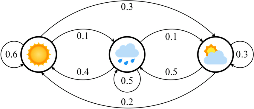
Interpretations:
If it's sunny today, it's 60% likely tomorrow will be sunny
If it's cloudy today, it's 50% likely tomorrow will be rainy
After today, you should have a better understanding of
The concept of Markov models and how they describe sequential dependencies
First order
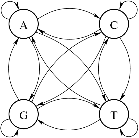
A Markov model can predict the next nucleotide depending only on the current nucleotide
Transition Probabilities: P(A∣G)P(A | G)P(A∣G), P(T∣C)P(T | C)P(T∣C), etc.
- Example: If a G is present, what is the probability the next base is A?
The likelihood of observing a nucleotide should depend on the preceding nucleotide
States: {A, C, G, T} – The four nucleotides.
0.3
0.2
0.3
0.2
0.2
0.3
0.1
0.4
0.4
0.1
0.4
0.1
0.1
0.3
0.2
0.4
Transition matrices help quantify nucleotide dependencies in sequences
| A | C | G | T | |
|---|---|---|---|---|
| A | 0.3 | 0.2 | 0.3 | 0.2 |
| C | 0.2 | 0.3 | 0.1 | 0.4 |
| G | 0.4 | 0.1 | 0.4 | 0.1 |
| T | 0.1 | 0.3 | 0.2 | 0.4 |
Instead of a graph, we can represent this as a transition matrix
Interpretation:
- If the current base is G, the probability of transitioning to C is 0.1.
- If the current base is A, there’s a 30% chance the next base is also A.
Current
Next
Example: Transition probabilities differ between coding and non-coding regions based on GC content
Genes (i.e., coding regions) generally have high GC content due to codon biases
Thus, we could assume that coding regions have higher P(G∣C) and P(C∣G)P(C | G)P(C∣G)
Non-coding regions would then have more random nucleotide distributions with less GC bias
| A | C | G | T | |
|---|---|---|---|---|
| A | 0.2 | 0.3 | 0.4 | 0.1 |
| C | 0.1 | 0.4 | 0.3 | 0.2 |
| G | 0.1 | 0.4 | 0.4 | 0.1 |
| T | 0.1 | 0.3 | 0.4 | 0.2 |
Current
Next
| A | C | G | T | |
|---|---|---|---|---|
| A | 0.3 | 0.2 | 0.3 | 0.2 |
| C | 0.2 | 0.3 | 0.1 | 0.4 |
| G | 0.4 | 0.1 | 0.4 | 0.1 |
| T | 0.1 | 0.3 | 0.2 | 0.4 |
Current
Next
By comparing transition probabilities, we can classify a sequence as coding or non-coding
P(S | C) = P(s_1 | C) \prod_{i=2}^{n} P(s_i | s_{i-1}, C)
P(S | N) = P(s_1 | N) \prod_{i=2}^{n} P(s_i | s_{i-1}, N)
Step 1: Train two Markov models—one for coding DNA and one for non-coding DNA.
Step 2: Compute the probability of the observed sequence (S) if it's
Coding (C)
Non-coding (N)
Step 3: Assign the sequence to the model with the higher likelihood
P(S | C)
P(S | N)
versus
or
If this sequence follows a C or N pattern, the probability will be higher
First-order Markov models classify sequences based on single nucleotide transitions, ignoring codon structure
Limited Context Awareness: FOMMs consider only the immediately preceding nucleotide, preventing them from capturing the inherent triplet codon structure of protein-coding sequences.
Frame-Shift Misclassification: Sequences that deviate from typical single-nucleotide transitions, such as those affected by insertions or deletions, may be incorrectly classified, leading to misidentification of coding regions.
Randomized Nucleotide Transitions: Since transitions occur between individual bases rather than codons, FOMMs do not distinguish between meaningful codon sequences and arbitrary base order.
After today, you should have a better understanding of
The concept of Markov models and how they describe sequential dependencies
Higher order
A higher-order Markov model (HOMM) improves gene prediction by modeling codon triplets
A k-th order Markov model considers k previous nucleotides when predicting the next k
A third-order Markov Model is codon-based
| ATG | CCT | GTA | TTA | |
|---|---|---|---|---|
| ATG | 0.2 | 0.3 | 0.4 | 0.1 |
| CCT | 0.1 | 0.4 | 0.3 | 0.2 |
| GTA | 0.1 | 0.4 | 0.4 | 0.1 |
| TTA | 0.1 | 0.3 | 0.4 | 0.2 |
Current
Next
Transition probabilities reflect valid codon structures, ensuring a more biologically accurate model
Models capture statistical biases inherent in real genes, such as the rarity of stop codons within coding regions
(Not all of them)
HOMMs are inefficient due to comparing between N models
We can bake in the idea that the region (i.e., coding or non-coding) influences codon transitions directly into one model
P(S | C) = P(s_1 | C) \prod_{i=2}^{n} P(s_i | s_{i-1}, C)
P(S | N) = P(s_1 | N) \prod_{i=2}^{n} P(s_i | s_{i-1}, N)
Coding (C)
Non-coding (N)
or
After today, you should have a better understanding of
The structure and purpose of Hidden Markov Models (HMM) in gene prediction
Hidden Markov Models (HMMs) solve the limitations of Markov models by introducing hidden states
Hidden States are biological states (e.g., coding vs. noncoding DNA) we are trying to determine
What we can still observe are k-mer transition probabilities in our genome
By directly including hidden states in our model, we can directly infer the optimal sequence of hidden states to explain our observed state transitions
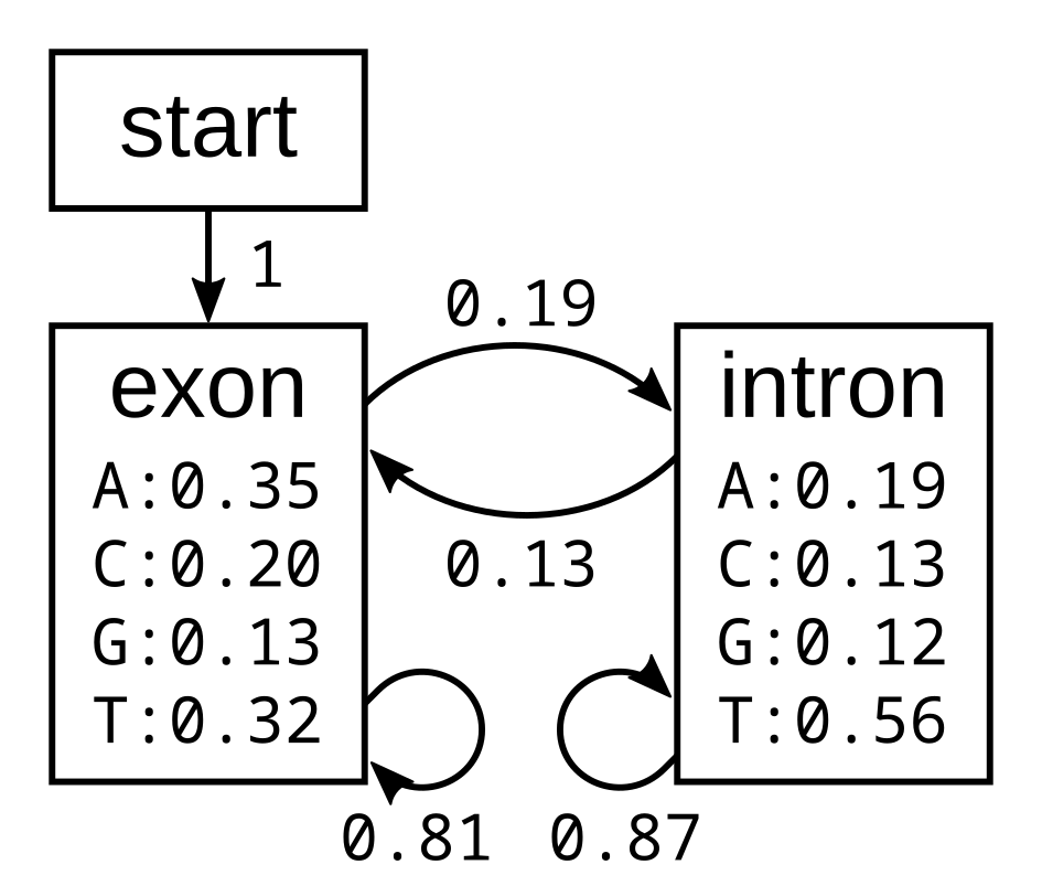
HMMs consist of states, transition probabilities, emission probabilities, and initial probabilities
States
- Hidden states: Coding vs. Non-coding DNA
- Observable states: Codons
Transition Probabilities
- Probability of moving from one hidden state to another.
- Example: P(coding→noncoding)P(\text{coding} \to \text{noncoding})P(coding→noncoding).
Emission Probabilities
- Probability of observing a nucleotide (A, C, G, T) in a given hidden state.
- Example: P(A∣coding)P(\text{A} | \text{coding})P(A∣coding), P(G∣noncoding)P(\text{G} | \text{noncoding})P(G∣noncoding).
After today, you should have a better understanding of
How to Predict Genes with an HMM
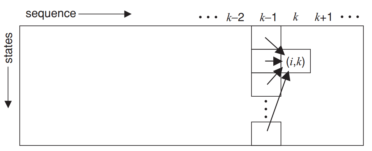
The Viterbi algorithm finds the most probable sequence of hidden states using dynamic programming
Instead of computing all possible paths, Viterbi keeps track of the best path so far.
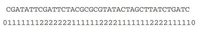
The Viterbi algorithm finds the best possible sequence of hidden states that explains the observed sequence
It is essential for determining which nucleotides belong to a gene
This is called dynamic programming, and we will cover this topic next week!
The Viterbi algorithm uses dynamic programming to efficiently compute the best state sequence
Step 1: Define Components
- States: Coding (C), Noncoding (N).
- Observations: A, C, G, T (DNA bases).
- Transition Probabilities: Probability of moving between states.
- Emission Probabilities: Probability of observing a base in a state.
Step 2: Initialize Probabilities
- Set initial probabilities for each state.
Step 4: Traceback
- Once the table is filled, we trace back to find the most probable path.
Step 3: Fill in the Table
- Compute probabilities step by step using previous best paths.
Before the next class, you should
Lecture 05A:
Sequence alignment -
Foundations
Lecture 04B:
Gene prediction -
Methodology
Today
Tuesday
BIOSC 1540: L04B (Gene prediction)
By aalexmmaldonado


