Computational Biology
(BIOSC 1540)
Apr 8, 2025
Lecture 13A
Cheminformatics
Foundations
Announcements
- Today is our last quiz
Assignments
Quizzes
Final exam
OMETs
- I will drop your lowest assignment if the response rate is 80% or higher.
- Current response rate: 63%
After today, you should have a better understanding of
Quiz 04
Please put away all materials as we distribute the quiz
Fill out the cover page, and do not start yet
Sit with an empty seat between you and your neighbors for the quiz
Quiz ends around 9:55 am
When you are finished, please hold on to your quiz and feel free to doodle or write anything on the last page
After today, you should have a better understanding of
Ligand-based drug design
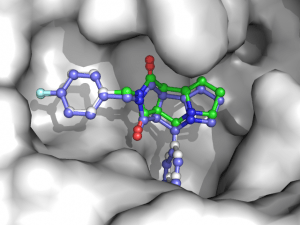
Structural insight into a disease is a privilege
Phenotypic drug screening involves testing compounds on an organism level to identify potential leads
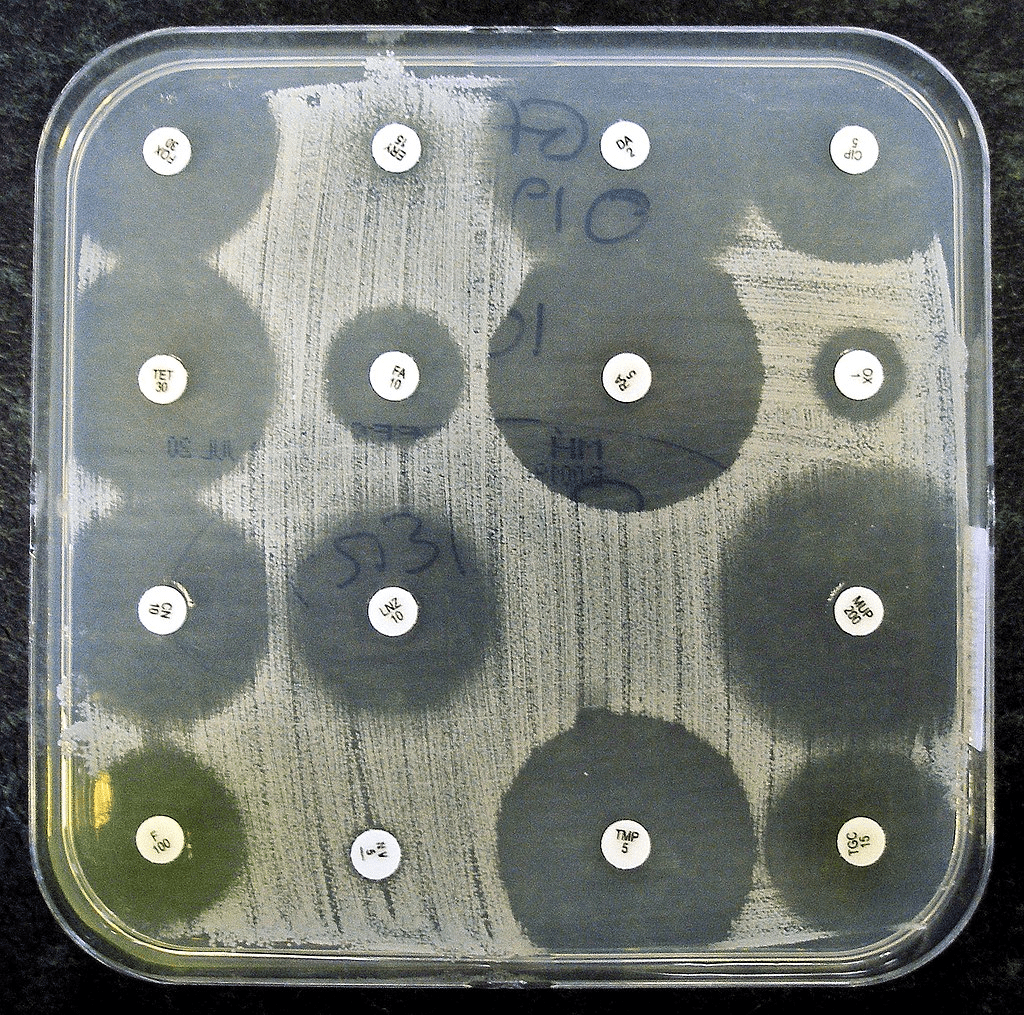
Example: Drug screening on an antibiotic-resistant bacterial strain to identify potential new leads
LBDD uses known compounds to guide drug discovery
Ligand-based drug design (LBDD) relies on the properties of known bioactive compounds
LBDD does not require the structure of the target protein, making it useful when this is unknown
Assumption: Similar structures can lead to similar—hopefully improved—biological effects
Motivation: If we find compounds with little bioactivity, we can use LBDD to find compounds with similar chemical features to improve specific outcomes

Key differences between structure- and ligand-based drug design
Structure-Based Drug Design:
- Requires 3D structure of the target protein.
- Uses the binding site structure to model potential interactions.
- Often employs docking and molecular simulations.
Ligand-Based Drug Design:
- Requires no structural information of the target.
- Uses the chemical structure and activity of known ligands as guides.
- Relies on molecular similarity rather than direct binding predictions.
Chemical space exploration is still challenging, and now we need to identify similar compounds
After today, you should have a better understanding of
Molecular properties
Molecular properties are used to predict how a compound behaves in the body, before any biological testing
These properties help prioritize molecules for synthesis and testing by estimating solubility, permeability, bioavailability, and toxicity.
LogP quantifies lipophilicity, which affects absorption, distribution, and membrane permeability
LogP is the logarithm of a compound’s partition coefficient between octanol and water.
High LogP values indicate lipophilic (fat-loving) molecules that may permeate membranes more easily, but also may have poor solubility and toxicity risks.
Low LogP values mean hydrophilicity (water-loving), which helps with solubility but may hinder permeability.
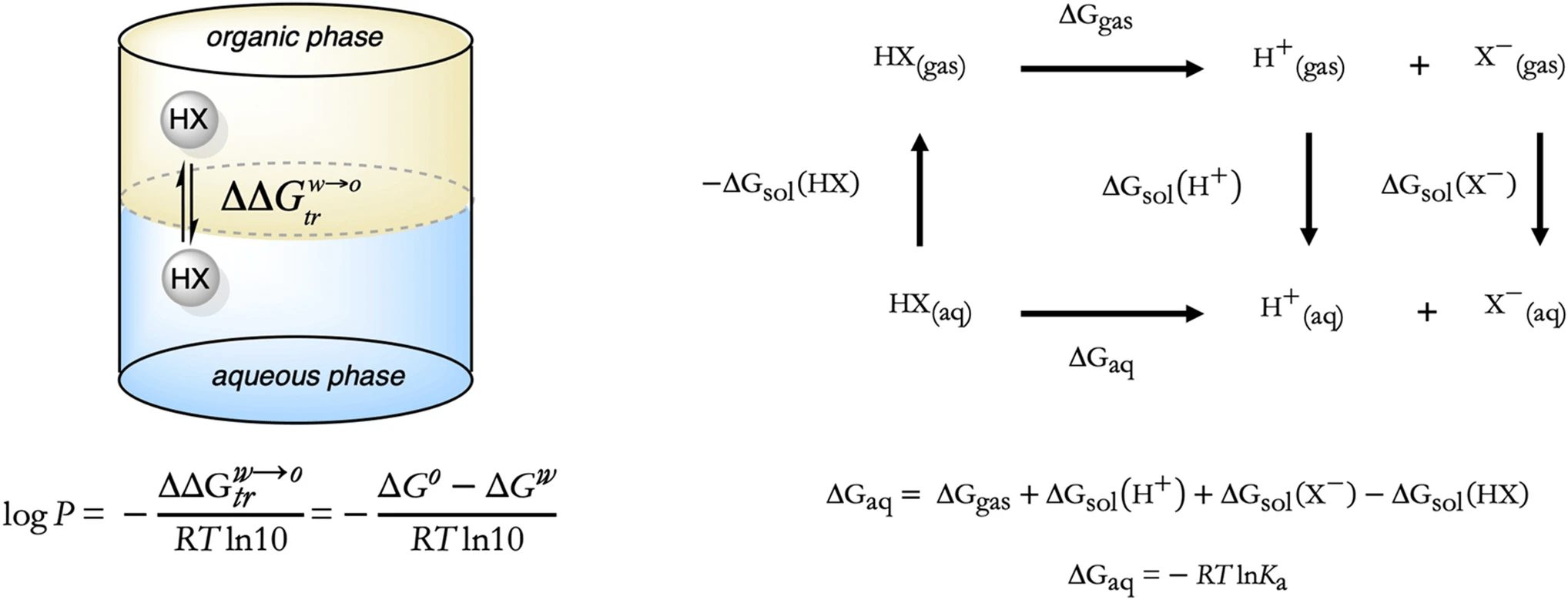
\log P = \log_{10} \left( \frac{[\text{solute}]_{\text{octanol}}}{[\text{solute}]_{\text{water}}} \right)
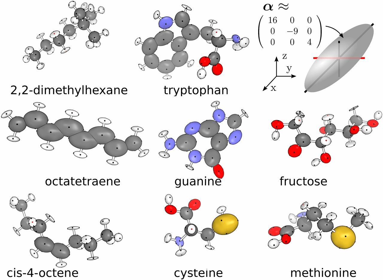
Molar refractivity (MR) measures polarizability and molecular volume
It is also used as a proxy for molecular volume—important in steric compatibility with binding pockets.
MR depends on molecular size and the type of atoms present.
Higher MR suggests greater polarizability, which can enhance binding via dispersion forces.
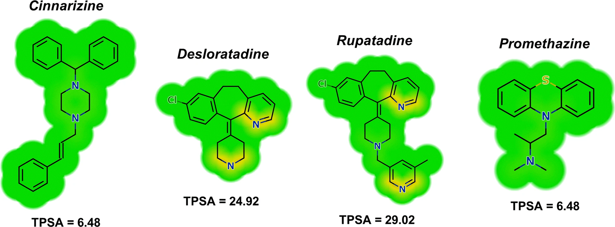
Topological Polar Surface Area (TPSA) predicts membrane permeability
Lower TPSA values (<90 Ų) suggest good potential for crossing the blood-brain barrier (BBB).
It is calculated from the surface area of oxygen and nitrogen atoms (and their attached hydrogens).
Molecules with TPSA >140 Ų typically show poor oral bioavailability.
Rotatable bonds contribute to molecular flexibility
Drug-like molecules often have fewer than 10 rotatable bonds.
Fewer rotatable bonds generally mean better oral bioavailability and metabolic stability.
Highly flexible molecules may pay a greater entropic cost upon binding, reducing affinity.

While molecular properties provide crucial insight, they do not fully describe a molecule’s structure or function
Two compounds can have similar LogP, TPSA, and molecular weights—but behave very differently due to subtle structural variations (e.g., isomers or stereochemistry).
Properties are global summaries, but molecular similarity often depends on local structural features like functional groups, ring systems, or atom connectivity.
After today, you should have a better understanding of
Molecular similarity
Quantifying molecular similarity is challenging
Which group of molecules should we pursue for increased bioafinity?
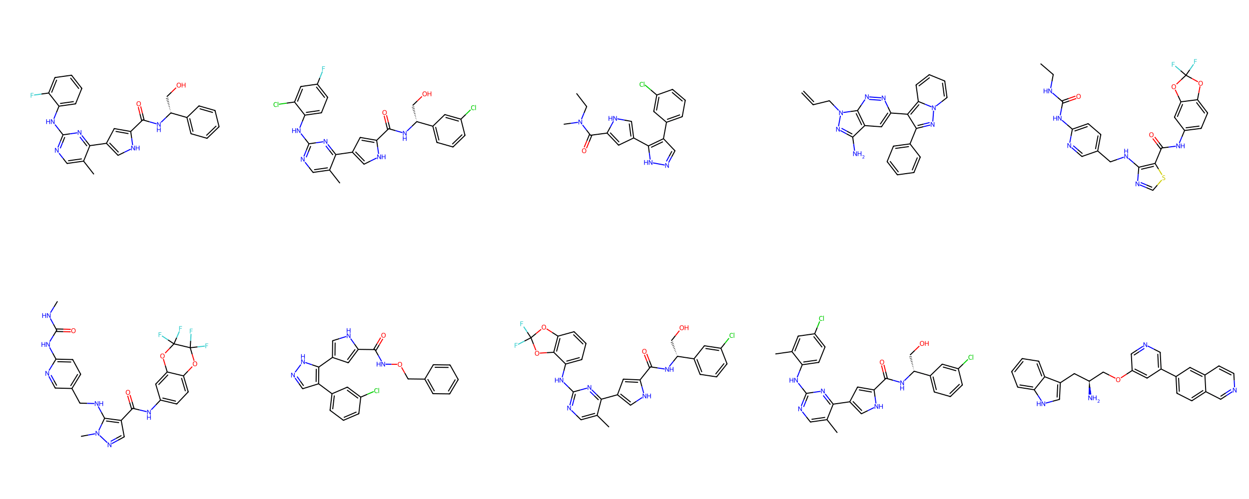
With your neighbors, determine how you would choose the group of molecules to pursue.
Suppose we performed an experimental high-throughput screen and identified these
potential leads
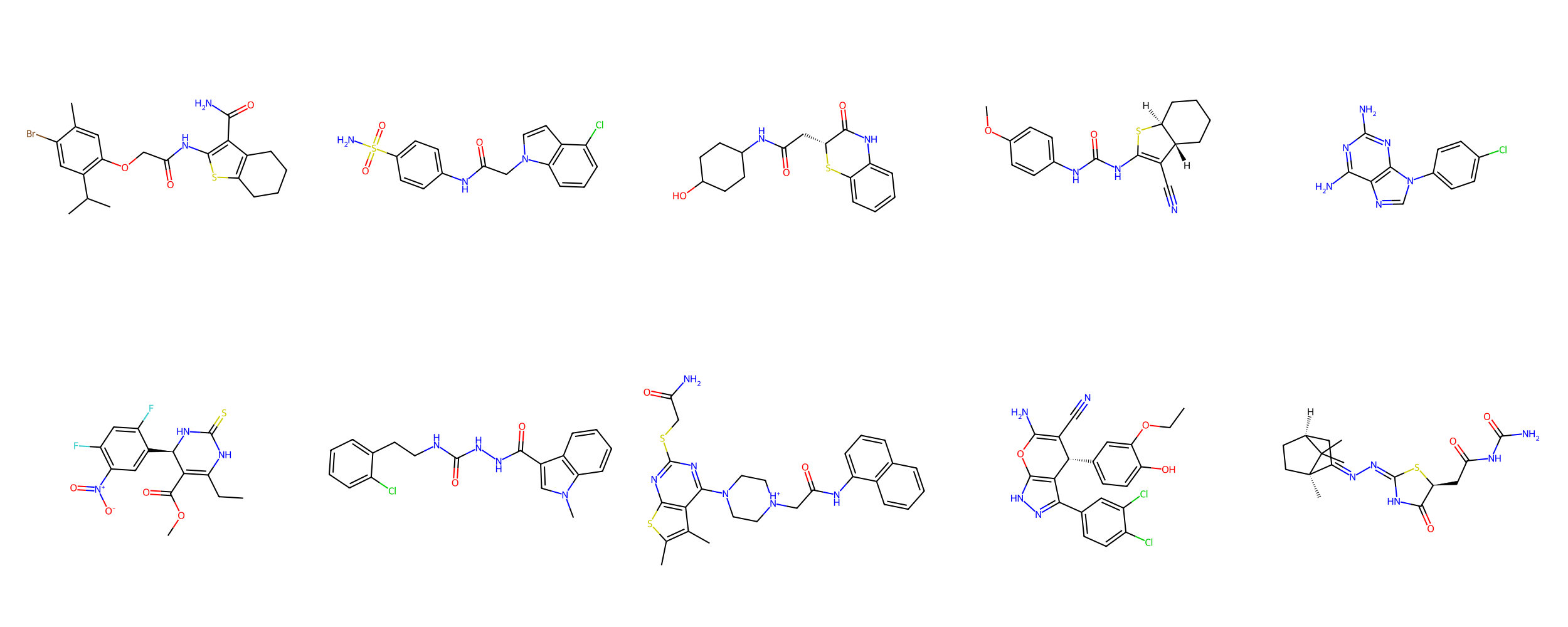
Group A
Group B

Molecular descriptors numerically encode chemical properties
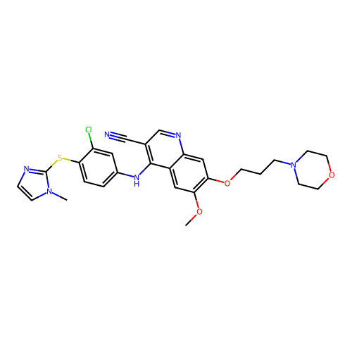
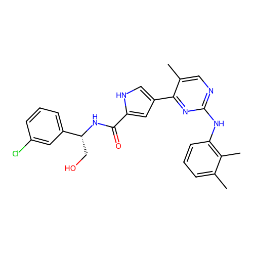
Computed with SwissADME
Molecular weight
565.09 g/mol
475.97 g/mol
Indicates the overall size of the molecule, impacting drug distribution and elimination rates in the body.
LogP
4.08
4.30
Measures lipophilicity, which influences a molecule's ability to cross cell membranes and affects absorption and bioavailability.
Molar Refractivity
156.23
134.72
Relates to polarizability and electron cloud distribution, affecting intermolecular interactions and binding affinity.
TPSA
122.76 Ų
102.93 Ų
Estimates the molecule’s ability to form hydrogen bonds, impacting solubility and permeability across biological membranes.
Num. rotatable bonds
10
8
Reflects molecular flexibility, which can influence binding affinity and oral bioavailability.
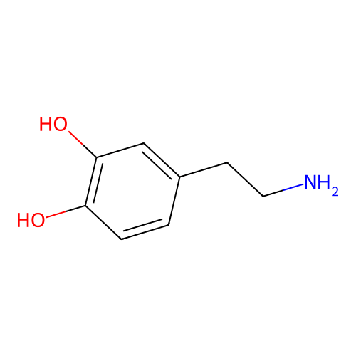
Molecules can have similar properties, with slight structural differences causing widely different functions
Computed with SwissADME
is a synthetic compound that acts as a vasoconstrictor by stimulating alpha-adrenergic receptors
Phenylephrine
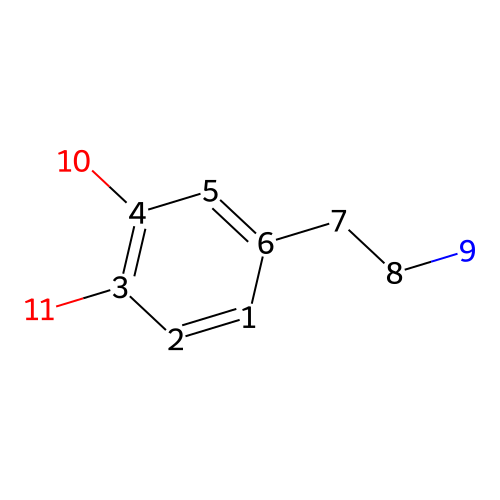
is a naturally occurring neurotransmitter in the brain and interacts with dopamine receptors
Dopamine
Simple descriptor comparisons are not sufficient for computing molecular similarity
Phenylephrine
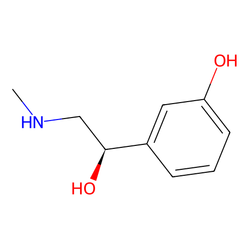
Dopamine
Molecular weight
LogP
Molar Refractivity
TPSA
Num. rotatable bonds
Molecular weight
LogP
Molar Refractivity
TPSA
SMILES
167.21 g/mol
0.65
47.01
52.49 Ų
3
CNC[C@@H](C1=CC(=CC=C1)O)O153.18 g/mol
0.46
42.97
66.48 Ų
2
C1=CC(=C(C=C1CCN)O)OMolecular fingerprints encode structural information
Phenylephrine
Dopamine
Extended Connectivity Fingerprints (ECFPs) encode structural features into numerical representations
10011000000000000001000000000000000000000000000000000000000000000000000000000000000000000000000000000000000000000000000000000000000000000000000000000000000000000000000000000000000000000000000000000000000000000000000000000010000010000000000000000000010000000000000000000000000000000000000000000000000000000000100000000000100000000000000000000000000000000000000000000000001000000000000000000000000000000000000000100000000000000000100000000000000000000000000000000000000000000000000000000000000000000000000000000000000000000000000000001000000000000000000000000000000000000000000000000000010000000000001000000000000000000010000000000000000000000000000000000000000000000000000000000000000000000000000000000000000000000000000100000000000000000000000000000000000000000000000000000000000000000000000000000000000000001000000000000100100000000000000000000000000001000000001000000100000000000000000000000000000001000000000000000010000000000000000000000000000000000000000000000000000000000000000000000000010000000000000000010010010000001001100000000000000100000000000000000000000000000000000000000000000000000000000000000000000000000000000000000000000000000000000000000000000000000000000000000000000000000000000000000000000000000000000000000000000000000000000000000000000000000000000000000000000000000000000000000000000000000000000000000000000000000000000000000000000100000000000000000000000000000000000000000000000000000000000000000000000000000000000000000000000010000000000000000000000000000000000000001000000010000001000000000000000000000000001000000000000000000000100000000000000000000000000000000000000000000000000000000000000000000000000000000000000000000000000000000000000000000000000000000000000000000000000000000000000000000000000000000000000000010000000000000000000000000100000000000000000000000000000000000000000000000000000000001000100000000010010100000000000000000000000000000000010000000000000000000000000000000000000000000100000000000000000000000000000000000000000000000000000000000000000000000000000000000000000001000000000000000001001000000000from rdkit import Chem
from rdkit.Chem import rdFingerprintGenerator
fmgen = rdFingerprintGenerator.GetMorganGenerator(
radius=3, fpSize=1024,
atomInvariantsGenerator=rdFingerprintGenerator.GetMorganFeatureAtomInvGen()
)
mol = Chem.MolFromSmiles("C1=CC(=C(C=C1CCN)O)O")
print(fmgen.GetFingerprint(mol))How do we compute this?
Hash functions are used to encode chemical information
For each heavy atom (i.e., not H), hash atom-specific properties
id10_iter0 = hash((6, 3, 0, 1))
print(id10_iter0)  # 7468469475583712974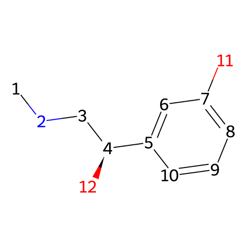
Let's look at carbons 6 and 10
Because of the same element and connectivity, they have the same ID0
id6_iter0 = hash((6, 3, 0, 1))
print(id6_iter0)  # 7468469475583712974
ID_0 = \text{hash}(Z_i, V_i, C_i, R_i, \ldots)
ID_0
Iteration 0 identifier
Z
V
C
R
Atomic number
Valence
Formal charge
Ring membership
"Encoding" is a computational term for transforming information in a numerical format for computers
For each additional iteration of n, incorporate the hashes of connected atoms that are n bonds away
Each iteration encodes local chemical information into each atom's ID
We can repeat the process for larger n, which captures more chemical information at a (small) computational cost
Repeat for all atoms while hashing n - 1 IDs
Next, encode the atom IDs that are exactly one bond away
id6_iter1 = hash((
    1, 7468469475583712974, # ID for atom 6
    2, 901285887933171736,  # ID for atom 5
    1, 901285887933171736   # ID for atom 7
))
print(id6_iter1)  # -1070477880882296059
Format:
(IterationNumber, AtomID, BondOrder1, AtomID1, BondOrder2, AtomID2, ...)id10_iter1 = hash((
1, 7468469475583712974, # ID for atom 10
1, 901285887933171736, # ID for atom 5
2, 7468469475583712974 # ID for atom 9
))
print(id10_iter1) # 9113858623660175530We keep track of atom IDs at each iteration to encode multiple "levels" of chemical information
# Iteration 0
[-96873481, -5237400, -608624, -40896092, 13106358, 39304191, 13106358, 39304191, 39304191, 39304191, 18495798, 18495798]

# Iteration 1
[-12887828, 34836456, -82428984, -76182021, 57441373, 18535308, 36698099, -16062189, -71082609, -16062189, -13803757, -35226747]

# Iteration 2
[-30242937, -22342045, -3701095, -83323106, -81401022, -79585126, 259777, -18164777, -83853893, -9624634, -63890015, -86218719]

# Iteration 3
[24482285, -67056973, -1049934, 58183281, 9686245, 65319696, -89546467, 90525418, -96278682, -31838946, -41820336, -42202112]
# Iteration 0
[39304191, 39304191, 13106358, 13106358, 39304191, 13106358, -608624, -608624, -2248911, 18495798, 18495798]
# Iteration 1
[-16062189, -16062189, -54942758, -54942758, 18535308, 80518135, -46276084, 85303560, -4225841, -13803757, -13803757]
# Iteration 2
[45202524, -32527659, 91315393, -86313403, 74663225, 43056615, -92441264, 61456743, 35268850, -86729888, -86729888]
# Iteration 3
[17051553, -83857497, -10864101, 42020134, 84228020, 88509243, 53634925, 58427327, 85169475, -62345869, -23012595]Similar structural features will share atom IDs
until our iteration starts incorporating different structural features

Atom IDs are encoded into a bit array
We can get a collection of atom IDs, but how would we rapidly compare molecules with different number of atoms?
We use bit arrays, which are fixed-length collections of ones and zeros
10101100 10101100
AND 11011010
--------
10001000
11011010This allows efficient operations
    10101100
OR  11011010
    --------
    11111110
Features that are in both molecules
Features that are in either molecules
Converting atom IDs to bit arrays
ecfp = [0, 0, 0, 0, ..., 0, 0, 0]-1070477880882296059 % 1024 = 908Decide on length of bit array, for example, 1024 and fill with zeros
Divide each atom ID by the length of the array and determine the remainder
Set the value of the bit array at that index to 1
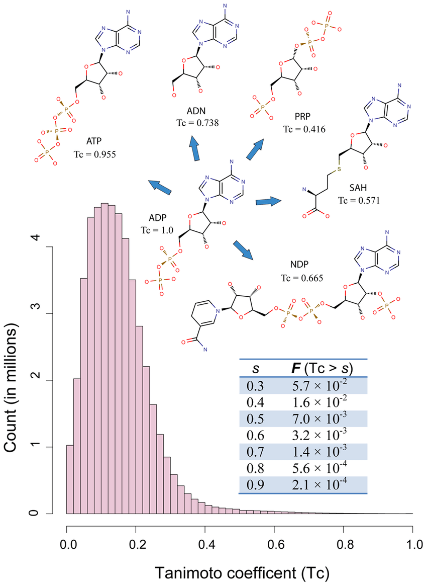
ecfp[908] = 110011000000000000001000000000000000000000000000000000000000000000000000000000000000000000000000000000000000000000000000000000000000000000000000000000000000000000000000000000000000000000000000000000000000000000000000000000010000010000000000000000000010000000000000000000000000000000000000000000000000000000000100000000000100000000000000000000000000000000000000000000000001000000000000000000000000000000000000000100000000000000000100000000000000000000000000000000000000000000000000000000000000000000000000000000000000000000000000000001000000000000000000000000000000000000000000000000000010000000000001000000000000000000010000000000000000000000000000000000000000000000000000000000000000000000000000000000000000000000000000100000000000000000000000000000000000000000000000000000000000000000000000000000000000000001000000000000100100000000000000000000000000001000000001000000100000000000000000000000000000001000000000000000010000000000000000000000000000000000000000000000000000000000000000000000000010000000000000000010010010000001001100000000000000100000000000000000000000000000000000000000000000000000000000000000000000000000000000000000000000000000000000000000000000000000000000000000000000000000000000000000000000000000000000000000000000000000000000000000000000000000000000000000000000000000000000000000000000000000000000000000000000000000000000000000000000100000000000000000000000000000000000000000000000000000000000000000000000000000000000000000000000010000000000000000000000000000000000000001000000010000001000000000000000000000000001000000000000000000000100000000000000000000000000000000000000000000000000000000000000000000000000000000000000000000000000000000000000000000000000000000000000000000000000000000000000000000000000000000000000000010000000000000000000000000100000000000000000000000000000000000000000000000000000000001000100000000010010100000000000000000000000000000000010000000000000000000000000000000000000000000100000000000000000000000000000000000000000000000000000000000000000000000000000000000000000001000000000000000001001000000000Tanimoto similarity compares the ECFPs between two molecules
Using bit operations, we can compute similarity using Tanimoto
\text{Tanimoto similarity} = \frac{c}{a + b - c}
- a is the number of bits set to 1 in vector A.
- bbb is the number of bits set to 1 in vector B.
- ccc is the number of bits set to 1 in both vectors A and B (the intersection).
This formula measures the ratio of the shared features to the total number of unique features between two molecules.
a = len(fp1_bits)
b = len(fp2_bits)
c = len(fp1_bits & fp2_bits)
Molecular similarity: The concept that similar molecules often show similar biological effects.
Tanimoto similarity ranges
Phenylephrine
Dopamine
How similar does ECFPs and Tanimoto say these molecules are?
After today, you should have a better understanding of
Quantitative structure-activity relationship (QSAR)
QSAR models link chemical structure with biological activity
Purpose: To predict the biological activity of molecules based on their structure.
Motivation:
- Reduces the need for experimental screening.
- Helps identify potential drugs quickly and cost-effectively.
Example: Predicting if a compound is likely to be an inhibitor of a target enzyme based on known inhibitors.
Types of QSAR Models:
- Linear Models: Simple, interpretable, e.g., linear regression.
- Nonlinear Models: Capture complex relationships, e.g., neural networks.
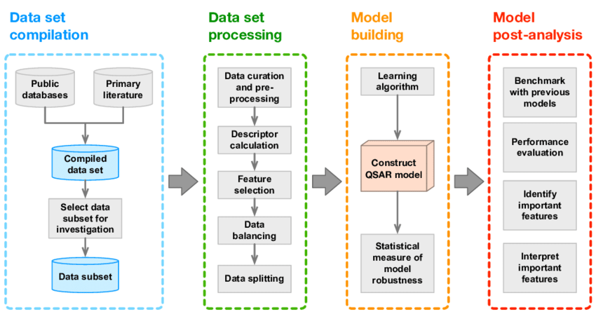
Developing a QSAR model follows systematic steps
- Data Collection: Gather biological activity and molecular data.
- Descriptor Calculation: Calculate numerical descriptors for each molecule.
- Model Selection and Training: Use machine learning to correlate descriptors with activity.
- Model Validation: Test model accuracy with independent datasets.
- Interpretation and Application: Use the model for predicting new molecules.
Linear regression models are simple but effective for QSAR analysis
Fits a linear relationship between descriptors and output
- Advantages: Easy to interpret.
- Limitations: Limited to linear relationships; struggles with complex datasets.
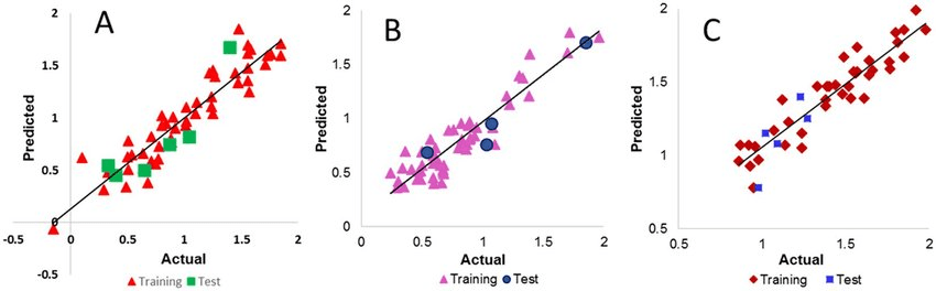
Y = \beta_0 + \beta_1 X_1 + \beta_2 X_2 + \ldots
Nonlinear models capture complex relationships in QSAR data
Examples of Nonlinear Models:
- Neural Networks: Capture complex, nonlinear patterns in large datasets.
- Random Forests: Effective for high-dimensional data, robust against overfitting.
Example: Predicting toxicity, where relationships between descriptors and outcomes are often nonlinear.
After today, you should have a better understanding of
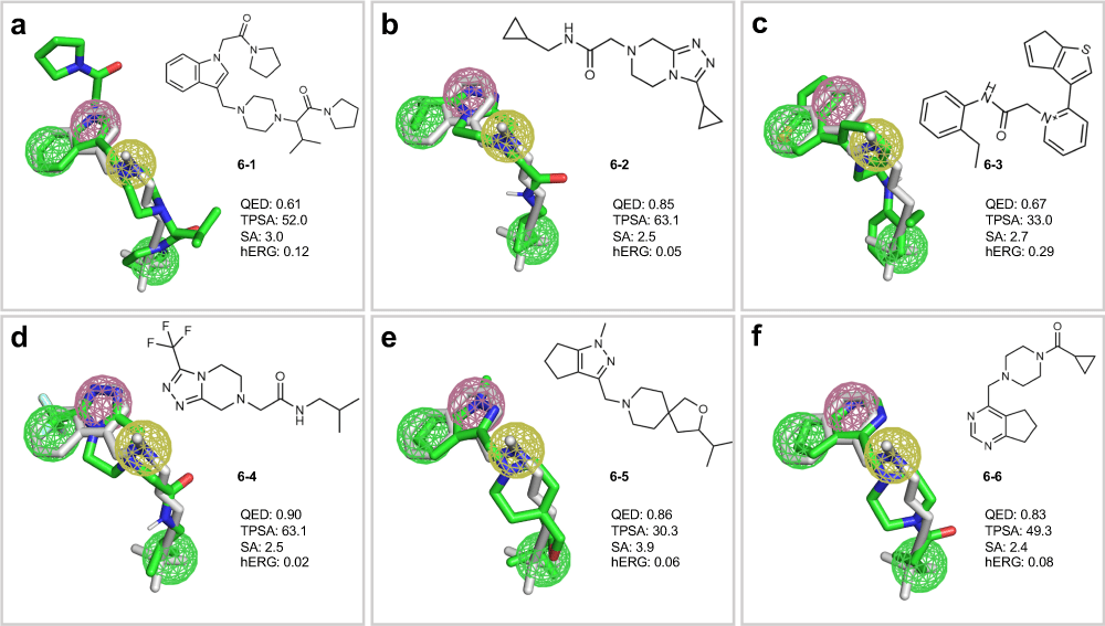
The role of pharmacophore modeling in identifying essential molecular features for activity.
Where QSAR quantifies activity, pharmacophore modeling identifies critical molecular features for activity
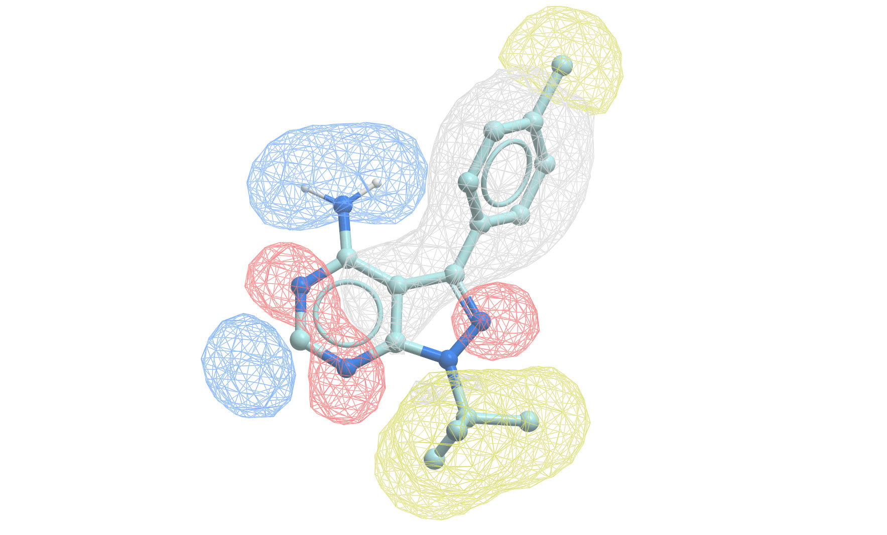
Pharmacophore modeling defines the essential features needed for biological activity
A pharmacophore is the 3D arrangement of molecular features required for biological activity
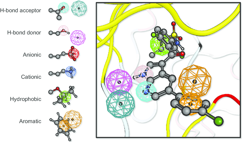
Building a pharmacophore model requires multiple active compounds
Step 1: Align active molecules
- Identify common structural features
- Determine spatial relationships
- Consider multiple conformations
Step 2: Define feature locations
- Mark shared pharmacophoric points
- Establish distance constraints
- Set tolerance spheres
Before the next class, you should
Lecture 13B:
Cheminformatics -
Methodology
Lecture 13A:
Cheminformatics -
Foundations
Today
Thursday
BIOSC 1540: L13A (Cheminformatics)
By aalexmmaldonado


