Local Composition Models
CHE 2101 - Spring 2022
April 21, 2022
Reference material: Rowley chapters 5 and 9
Lecture 25
van der Waals Mixture Partition Function
Learning Objective
Partition functions are normalization constants
Expectation values of some property
Semi-classical partition function
What is the meaning of each term?
Molecular partition function
System partition function
Indistinguishability of molecules
Configurational partition function
Partition functions review
Configurational partition function
That makes sense, right?
Not to me
Partition functions review

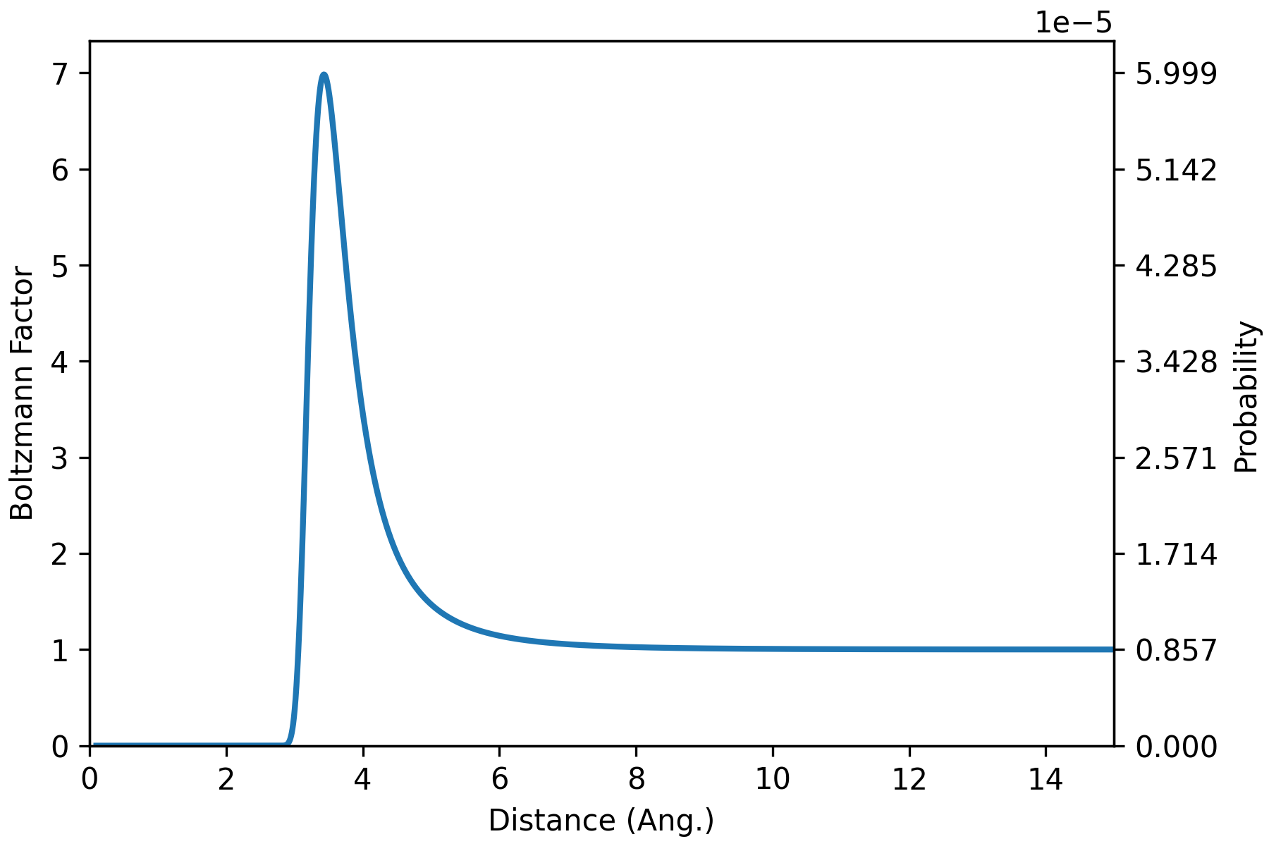
Configurational partition function - Toy system
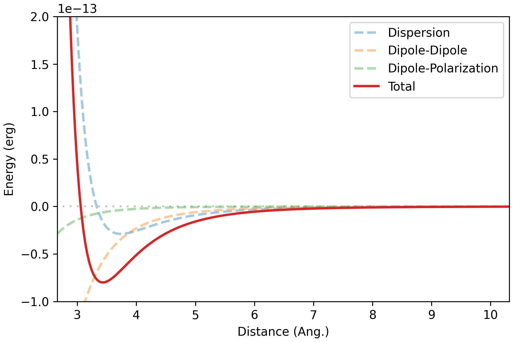
Angle-averaged interaction energy of water dimer (HW 7)

T = 298.15  # K
beta = 1/(kB * T)  # 1/erg
bolz_factor = np.exp(-beta*u_total)
Z = np.sum(bolz_factor)  # 116691.201
prob = bolz_factor/Z
Partition functions review
Partition functions review
Z for real systems would have 3N dimensions
Approximations are needed for analytical expressions
Configurational partition function - Real systems
For example: van der Waals partition function
Approximations/Approach
- Liquid molecules constrained in "lattice" cages
- Total potential energy is pairwise additive
- Mean-field pairwise potential
- No correlation between cages

Review from lecture 20
Partition functions review
Conceptualizing vdW framework
Lattice cage confining some molecule
Molecules do not respond to the motion of neighbors
(i.e., no correlation)
Review from lecture 20
Partition functions review
vdW partition function
- Free volume: Cage volume accessible to the center of the hard sphere
- Two parameters
- The exponential term is the lattice potential contribution
- The potential energy of a molecule exploring its cage
Lattice information
Molecular diameter
Averaged lattice potential
Review from lecture 20
Takeaways
- Analytical expressions for Z are challenging
- vdW partition functions provide a framework for approximating Z

I learned
this
You learned
this?
I learned
this
Alex
You
Helmholtz Free energy of Mixing
Learning Objective
Disclaimer: Assuming
Helmholtz free energy of mixing
- vDW partition function for mixtures
- , , all cancel leaving you with
Entropic effects based on free volume differences
Energetic differences between like and unlike interactions
Calculating
- Put final minus initial Helmholtz free energy in terms of partition functions
Helmholtz free energy of mixing
Possible assumption 1/2
Athermal contribution
Free volume is proportional to N
Use
Ideal mixture model
Would this be always positive, negative, or does it depend? Why?
Helmholtz free energy of mixing
Possible assumption 2/2
Athermal contribution
Define volume fraction as
Flory-Huggins Equation
Free volume if proportional to molar volume
Helmholtz free energy of mixing
Residual contribution
Direct expressions are rare, so we use this instead
Easy, right?
Local composition models can accomplish this
Now we just need to find
Ehh

Takeaways
- Use vdW partition function for Helmholtz free energy of mixing
- Ways to compute the athermal contribution
- Can use local composition models for residual contribution

I learned
this
You learned
this?
I learned
this
Alex
You
Local composition models
Learning Objective
Disclaimer: Assuming
Review: Pair correlation function
Configurational integrals for real systems are challenging
Relative probability of finding a second molecule some distance away

Pair correlation function ( ) is a proxy for configurational information

1
Distance
Coordnation shells
Review from lecture 20
Review: Pair correlation functions
Number of neighboring molecules

Differential number of atoms in a shell r distance away
is the numerical density of the system
is a volume element
Total number of atoms within a distance r
What happens if we integrate to ?
Review from lecture 20
Local composition models
Computing local compositions
Type 1
Type 2
Number of type 2 moleucles around type 1
Number of type 1 moleucles around type 2

Local composition models
Computing local compositions
We can use radial distribution functions to compute local mole fractions
For example, the mole fraction of type 1 molecules around another type 1

Local composition models
Computing local compositions
We can simplify this expression by considering differences in random mixing
Probability ratio of finding type 2 molecules over type 1
Example: 50:50 mixture
Number of neighboring molecules
Mixing factor
Local composition models
Circling back to
We can now estimate using this concept of nonrandom mixing factors
Wilson Model
Assumptions
- Potentials of mean force are used instead of pair potentials
- Shell thickness is the first coordination shell

Disclaimer: Assuming
Local composition models
Circling back to
Nonrandom two-liquid (NRTL) model
Introduces nonrandom mixture parameters

Disclaimer: Assuming
Local composition models
Activity coefficients
Both local models can compute acitivty coefficients
Wilson
NRTL
Takeaways (final)
- Pair correlation functions are a proxy for configurational information
- Deviations in spatial compositions provide information on nonideal mixing
- Local models can be used to compute activity coefficients and energy of mixing

I learned
this
You learned
this?
I learned
this
Alex
You
Local composition models
By aalexmmaldonado
Local composition models
- 346


