Circuit Complexity of Bipartite Matching in Bounded Planar Cutwidth Graphs
Aayush Ojha, 13807009
Thesis Supervisor:- Dr. Raghunath Tewari
M.Tech. Thesis Defence
Problem
\text{Circuit Complexity of Bipartite Matching in }
\text{Bounded Planar Cutwidth Graphs}
\text{Understanding of Input is crucial here }
\text{Exploit planarity and bounded planar cutwidth?}
\text{As circuit classes are very weak, }
\text{usually some advice is provided in input}
Known Results
\text{Lower Bound is } AC^0
\text{Upper Bound is } ACC^0
\text{Hansen et al.}
Motivation
- Barrington showed that Matching in Bounded Cutwidth Graphs is
NC^1\text{-complete}
ACC^0
AC^0
- Nice algebraic, graph-theoretic and geometric properties
- Hansen et al. conjectured that upper bound can be improved to
- For bounded planar cutwidth, Hansen et al. showed a better upper bound of
Preliminaries
Circuit Classes
| Circuit Class | Depth | Gates | Fanin |
|---|---|---|---|
| Unbounded | |||
|
|
Unbounded | ||
|
|
Unbounded | ||
| Bounded |
AC^0
O(1)
Mod_m
O(1)
AC^0[m]
ACC^0
O(1)
Mod_m \text{ } \forall m \in \mathbb{N}
NC^1
O(\log n)
\text{AND, OR, NOT}
\text{AND, OR, NOT}
\text{AND, OR, NOT}
\text{AND, OR, NOT}
Grid Graph and Concatenation
Grid Graph: Vertices on integral coordinate and edges are horizontal or vertical and of length 1
Monoid
\text{ A set } S \text{ and a binary operation } \oplus \text{ with properties:}
\text{Closure:}
\text{Associativity:}
\text{Identity:}
\text{Notation: } \mathcal{M}
a\oplus b = c \text{ and } a,b \in S \Rightarrow c \in S
(a \oplus b) \oplus c = a\oplus (b \oplus c)
\exists e \in S\text{, } \forall a \in S\text{, }e\oplus a =a \oplus e =a
Monoid
\text{Aperiodic: }
\mathcal{G} \subseteq \mathcal{M}, \text{ is a group then } \mid\mathcal{G}\mid = 1
\text{Solvable: }
\mathcal{G} \subseteq \mathcal{M}, \text{ is a group then }
\mathcal{G} \text{ is solvable}
Cutwidth
\text{Cut = 3}
\text{Cut = 2}
Cutwidth
\text{Cut = 2}
\text{Cutwidth=2}
Planar Cutwidth
Branching Programs
I(x,a,b) = \begin{cases}
a, & x=0\\
b, & x=1
\end{cases}
Instruction:
x \in \{0,1\}
a,b \in \mathcal{M}
\mathcal{M} \text{ is a Monoid}
Branching Programs
P=I(x_{i_1}, a_1,b_1)
I(x_{i_2}, a_2,b_2)
\cdots
I(x_{i_l}, a_l,b_l)
\mathcal{A} \subseteq \mathcal{M} \text{ be accepting set}
I(x_{i_j},a_j,b_j) = m_j
P \text{ accepts } x
\Longleftrightarrow m_1 m_2 \cdots m_l \in \mathcal{A}
x =x_1x_2 \ldots x_n \in \{0,1\}^{n}
Algebraic Characterization
L \text{ accepted by a monoid } \mathcal{M} \Longleftrightarrow
\text{L accepted by poly size Branching Program over } \mathcal{M}
\text{Monoid}
\text{Circuit Class}
AC^0
ACC^0
NC^1
\text{Aperiodic}
\text{Solvable}
\text{Non-solvable}
\text{ By Barrington and Therien}
Results on Reachability
\text{Barrington et al. showed reachability in }
\text{bounded width grid graphs is}
AC^0 \text{-complete}
\text{Proof exploits the nice geometric structure}
Assumptions on Input
- Odd length: Grid Graph is of odd length (odd number of columns)
Hansen et al. assumed following:
- Grid Graph Embedding: Graph is given as planar bounded width grid graph with embedding
- Implicit Bipartition: Bipartition of a vertex is determined by parity of sum of its coordinates
Assumptions on Input
- Odd length: If not bipartition of vertex changes on concatenation
AC^0[2]
NC^1\text{-complete}
Reasons for assumptions:
- Grid Graph Embedding: Getting planar embedding is
- Implicit Bipartition: Computing Bipartition is in
Our Contributions
\text{Bounded Planar Cutwidth Trees}
\text{Upper Bound: } AC^0[2]
\text{Bounded Planar Cutwidth Series-Parallel Graphs}
\text{Lower Bound: } AC^0
\text{Upper Bound: } AC^0 \text{ (Leaves in same bipartition)}
\text{Assumptions:}
\text{Grid embedding with implicit bipartition}
\text{Odd length not necessary}
\text{For Special Graphs}
Our Contributions
\text{Assumptions:}
\text{Grid Graph with diagonal edges}
\text{Bounded Planar Cutwidth Graphs:}
\text{Lower Bound: } \notin AC^0[p^\alpha]
p \text{ is an odd prime,}\alpha \in \mathbb{N}
\text{General Graphs}
\text{Proof Idea:}
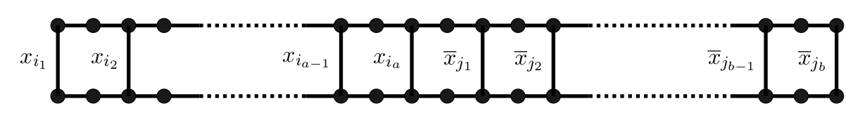
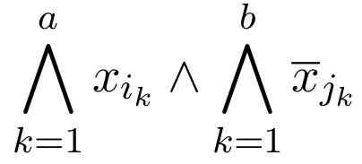
\text{Reduce } Parity \text{ to matching}
\text{Encode parity in bipartition of vertices}
\text{Implicit bipartition not necessary}
Upper Bounds for Trees
\text{Type M}
\text{Type U}
\text{Type } \Phi
Upper Bounds for Trees
\text{Type M}
\text{Type U}
\text{Type M}
Upper Bounds for Trees
\text{Type U}
\text{Type M}
Upper Bounds for Trees
\text{Type } \Phi
\text{Case 1}
Upper Bounds for Trees
\text{Type } \Phi
\text{Case 2}
Upper Bounds for Trees
\text{Type } \Phi \text{ ?}
\text{Can we give a simple criteria for }
\text{Case 1}
Upper Bounds for Trees
\text{Type } \Phi \text{ ?}
\text{Can we give a simple criteria for }
\text{Case 1}
Upper Bounds for Trees
\text{Node } v \text{ with two children subtrees}
\text{ having odd no. of vertices}
v
Upper Bounds for Trees
\text{Children Subtrees having odd no. of vertices?}
\text{Use Reachability and Parity}
\text{Thus, Upper Bound: } AC^0[2]
\text{Bounded width grid graph Reachability} \in AC^0
Upper Bounds for Trees
\text{Assuming, all leaves are in same bipartition}
\text{Criteria for Type } \Phi \text{ can be improved}
\text{Search for odd length path in tree}
\text{Thus, Upper Bound: } AC^0
Lower Bounds for SP Graphs
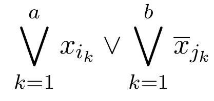
\text{ Every } AC^0 \text{ circuit computes either } \Sigma_d \text{ or } \Pi_d \text{ formula}
\text{Induction over } d
\text{Similar to Barrington et al. Lower Bound for Reachability}
\text{ in bounded width grid graphs}
Lower Bounds for SP Graphs
\text{Base Case:}
\Sigma_1:
\Pi_1:
Lower Bounds for SP Graphs
\text{Inductive Step:}
\Sigma_d:
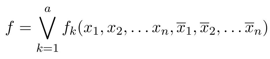
f_k \text{ } \rightarrow
\text{ } G_k
Lower Bounds for SP Graphs
\text{Inductive Step:}
\Pi_d:
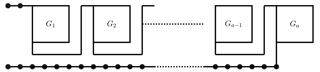
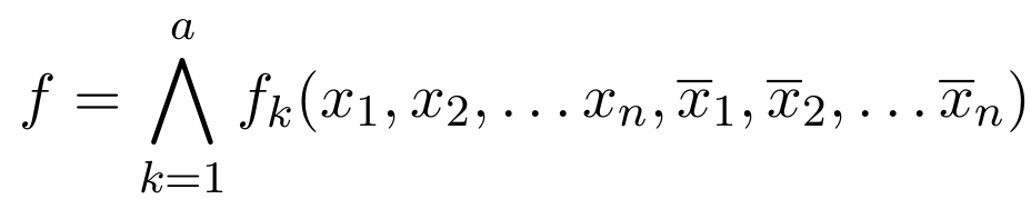
f_k \text{ } \rightarrow
\text{ } G_k
Conclusion & Future Work
- Better results for trees.
- Lower Bound for SP Graphs suggests that upper bound for trees in quite tight
- Hansen's conjecture is still unresolved
- Lower Bound for Trees
- Better upper bounds for other classes of graphs
References
Thank You
Proof for upper bound
ACC^0

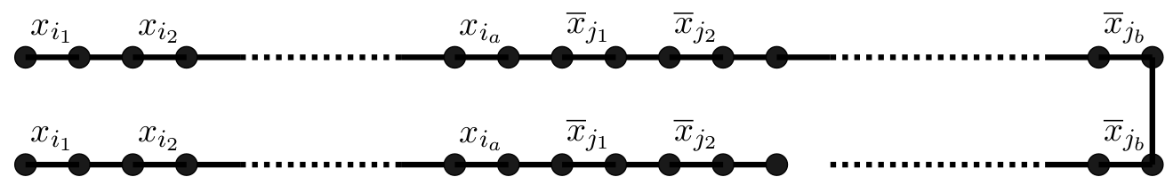
Visualize graph as concatenation of smaller grid Graphs
Proof for upper bound
ACC^0
Reduce graphs to a Monoid

G
(X,Y,R) = G^{\mathcal{M}}
X \text{ is leftmost column of } G
Y \text{ is rightmost column of } G
R \text{ is a binary relation between}
2^{X} \text{ and } 2^Y
Proof for upper bound
ACC^0
Reduce graphs to a Monoid
(X,Y,R)
R \text{ is a binary relation between}
2^{X} \text{ and } 2^Y
(x,y) \in R \text{ if } G-\overline{x}-y \text{ has perfect matching}
x \subseteq X \text{, } y \subseteq Y
(x,z) \in RS \Longleftrightarrow \exists y \text{ s.t.} (x,y) \in R \text{ and }(y,z) \in S
\text{We define } RS \text{ for two relations } R,S
Proof for upper bound
ACC^0
Monoid Product
\text{We add } 1 \text{ and } 0 \text{ to monoid}
(X,Y,R_1)(Y,Z,R_2) = (X,Z,R_1R_2)
0x = x0 = 0
(X,Y,R)(U,V,S) = 0
1 x = x = x1
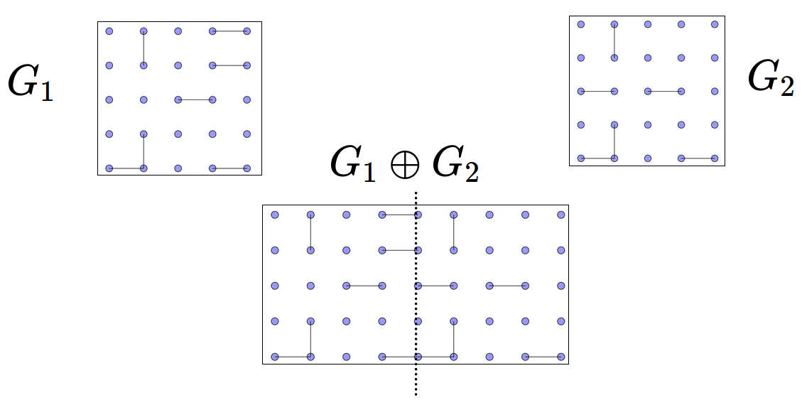
Monoid Product and Graph Concatenation
(G_1 \oplus G_2)^{\mathcal{M}} = G_1^{\mathcal{M}}G_2^{\mathcal{M}}
Proof for upper bound
ACC^0
Monoid Product and Graph Concatenation
(G_1 \oplus G_2)^{\mathcal{M}} = G_1^{\mathcal{M}}G_2^{\mathcal{M}}
G = G_1 \oplus G_2 \oplus G_3 \oplus G_4
G^{\mathcal{M}} =G_1^{\mathcal{M}} G_2^{\mathcal{M}} G_3^{\mathcal{M}} G_4^{\mathcal{M}}
Use Branching Program
Proof for upper bound
ACC^0
Use Branching Program
All that is left is to show that monoid is solvable
Requires Graph-theoretic analysis
For Simplicity, we skip further details
Thesis Presentation
By Aayush Ojha