{light_pred}
University of Bologna
1
Smart Home Dataset Research & Selection
2
Exploratory Data Analysis (EDA) & Quality Assessment
3
Definition of Methodological Approaches
5
Advanced Modeling & Data Refinement strategies
4
Baseline Implementation: Probabilistic Nowcasting
6
Performance Evaluation & Discussion of Limitations
Project Roadmap
The Dataset
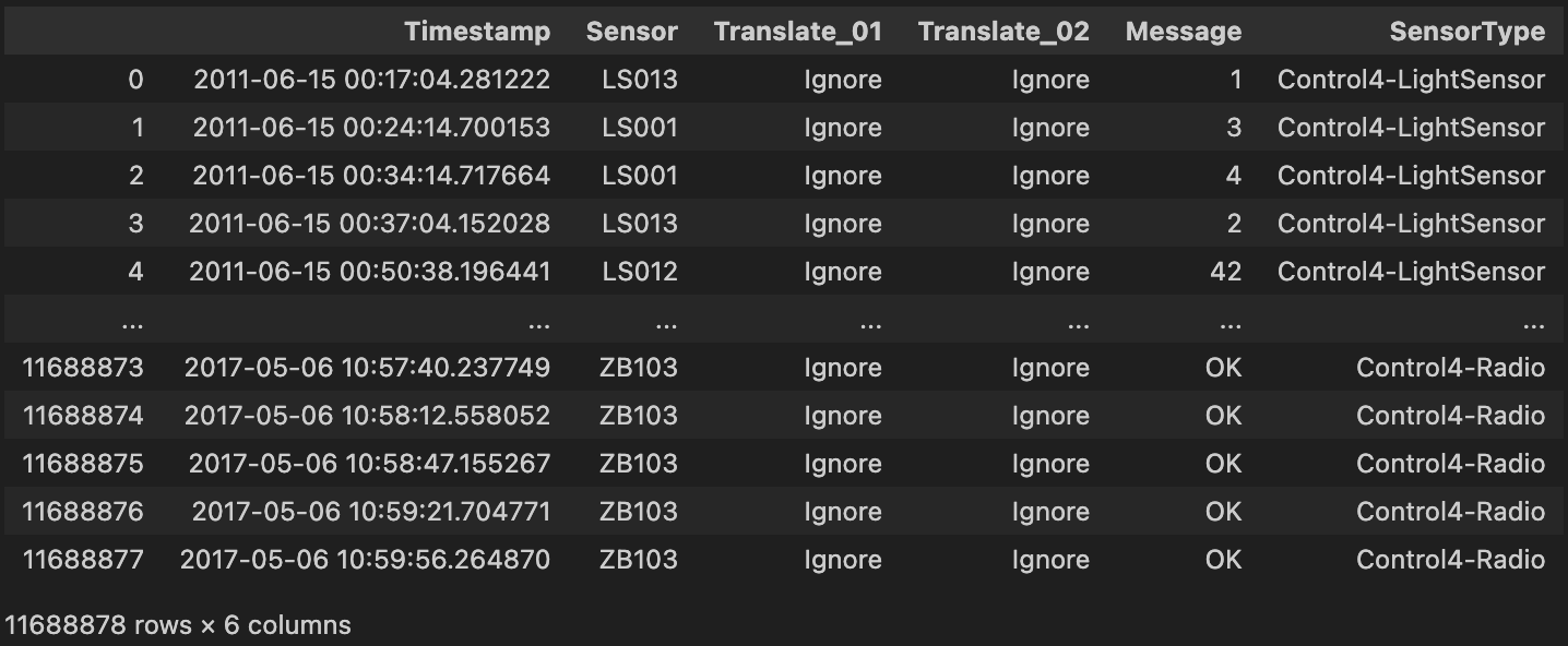
- Raw dataset sourced from UCI ML Repository: smart home sensor stream (house csh114).
- 11.7 million events spanning from June 2011 to May 2017.
- Sensors:
- Lights
- Motion detectors
- Doors
- Buttons
- Light sensors
- Temperature
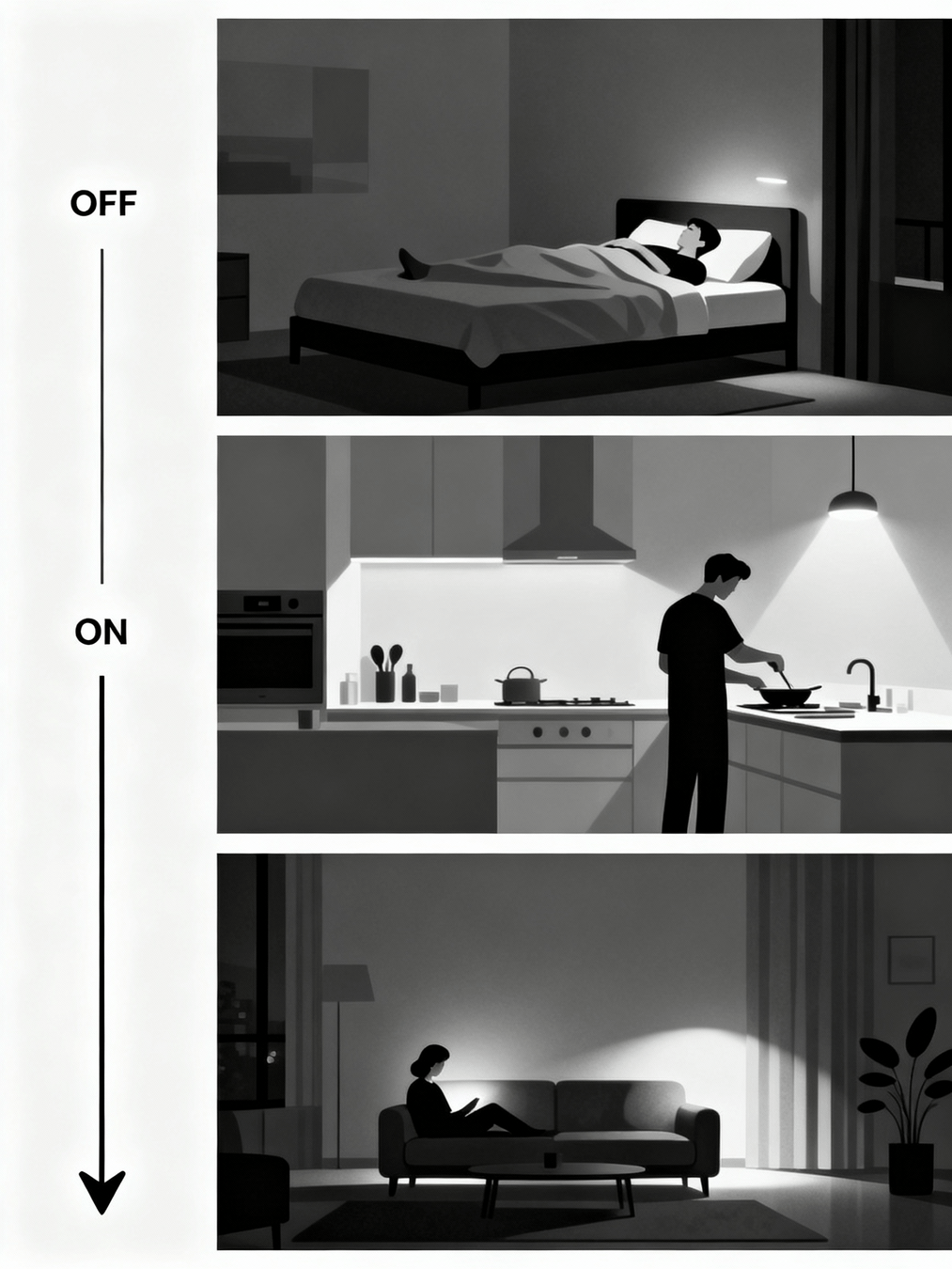
# DATASET
The sensors
-
Motion Sensors 🟢 (useful)
- PIR motion detectors with light sensors that detect presence and ambient brightness (0-100 range)
-
Door Sensors 🟢 (useful)
- Magnetic reed switches that report OPEN/CLOSE states for doors and cabinets
-
Temperature Sensors 🟠 (not informative)
- Built into door packages, measure ambient temperature with 0.5°C accuracy
-
Light Switches 🟢 (useful)
- Report brightness levels (0-100) and capture dimmer adjustment
-
Light Sensors 🟡 (proxy)
- Photocell sensors that measure ambient brightness levels (0-100 range)
-
Button Sensors 🟡 (proxy)
- Capture user interactions with switches including taps, holds, and tap counts
-
Battery Monitors 🔴 (independent)
- Track power levels (0-100%) for all battery-operated sensor
# DATASET
Loading Datataset
home = 'csh114'
path_home = root_data + '/' + home + '.rawdata.txt'
df = pd.read_csv(path_home, sep='\t', header=None, names=col_names)

df = df[df['Timestamp'] <= '2014-11-18']

df
# PRESENTING CODE
Time filtering
home = 'csh114'
path_home = root_data + '/' + home + '.rawdata.txt'
df = pd.read_csv(path_home, sep='\t', header=None, names=col_names)

df = df[df['Timestamp'] <= '2014-11-18']

df
# PRESENTING CODE
Raw Dataset
home = 'csh114'
path_home = root_data + '/' + home + '.rawdata.txt'
df = pd.read_csv(path_home, sep='\t', header=None, names=col_names)

df = df[df['Timestamp'] <= '2014-11-18']

df
# PRESENTING CODE
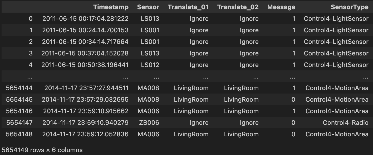
Data Cleaning
def normalize_message(msg):

    if msg == 'OPEN':
        return 1
    elif msg == 'CLOSE':
        return 0
    elif msg == 'ON':
        return 1
    elif msg == 'OFF':
        return 0
    try:
        val = float(msg)
        return 1 if val > 0 else 0
    except (ValueError, TypeError):
        return 0
# PRESENTING CODE
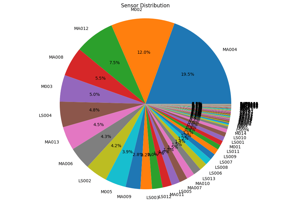
# DATA EXPLORATION
Sensors distribution
Comprehensive frequency analysis across all 64 sensors with identification of dominant contributors.
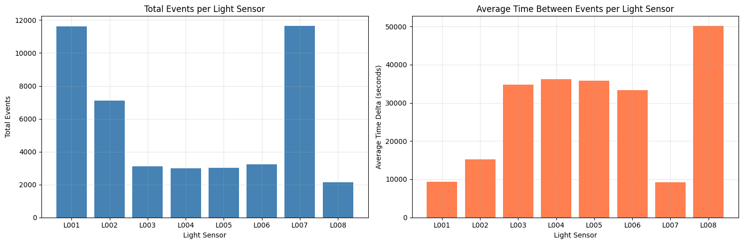
Lights and Gaps distributions
Number of total events of each light on the left and average time between light-events.
# DATA EXPLORATION
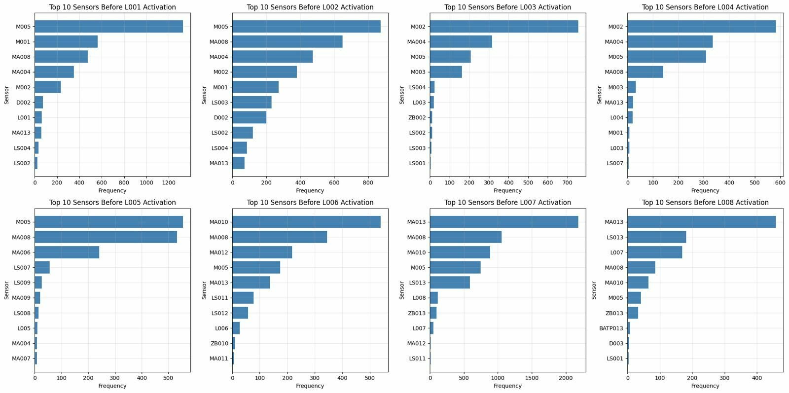
10 most frequent sensors
Ten most frequent sensors immediately before light activation.
# DATA EXPLORATION
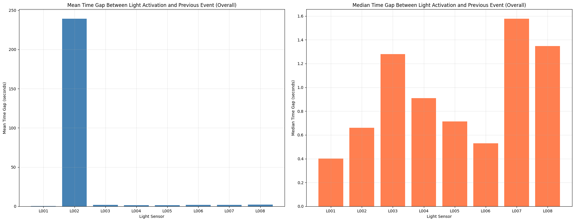
Previous sensor mean time gap
Average time gap between light activation and previous event overall.
# DATA EXPLORATION
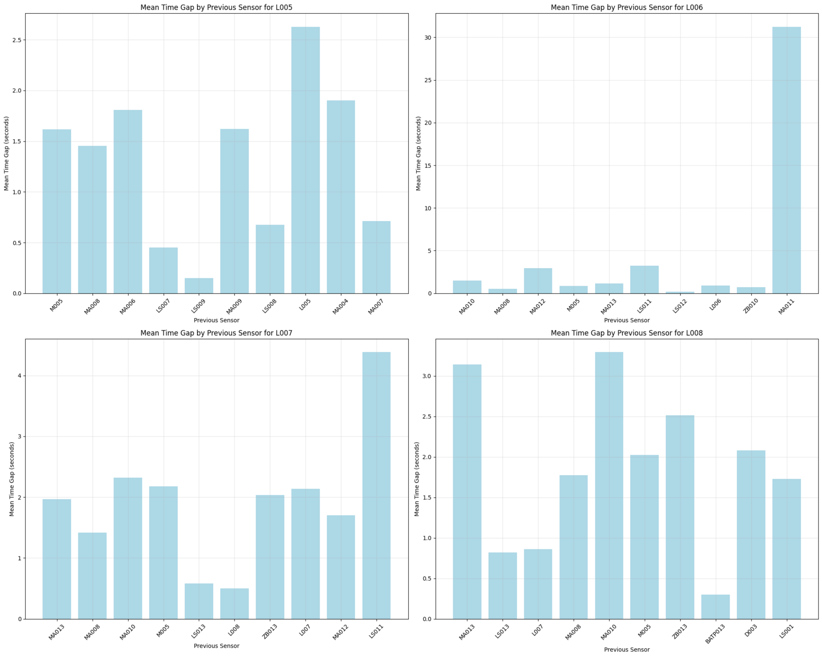
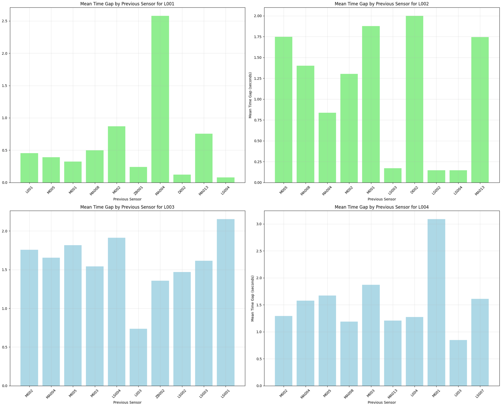
Previous sensor mean time gap
Mean time gap between light activation and previous event for each light.
# DATA EXPLORATION
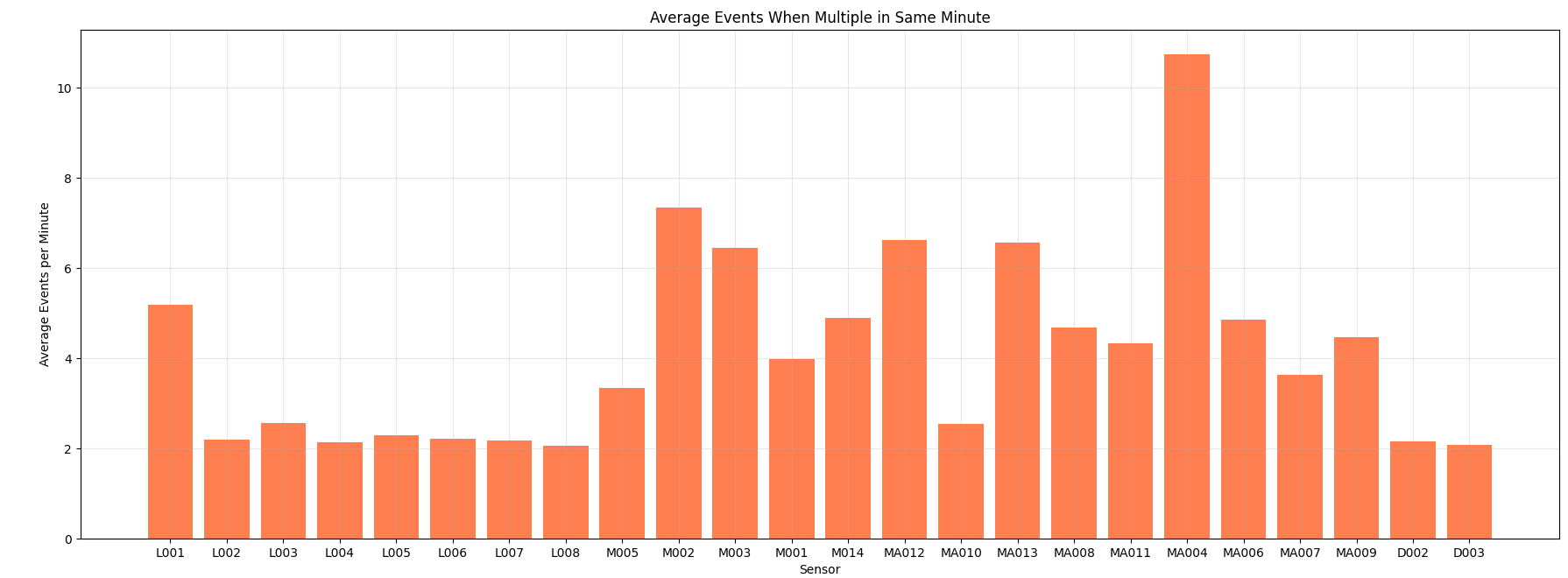
Same event - Same minute
Average number of sensor-event repetition in the same minute.
# DATA EXPLORATION
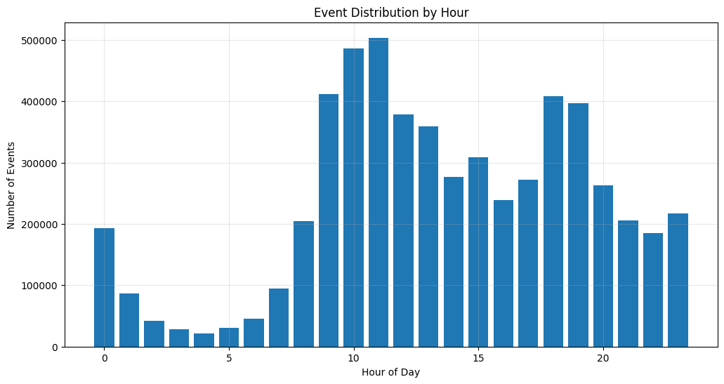
Event distribution by Hour
Histogram of events based on hour of the day.
# DATA EXPLORATION
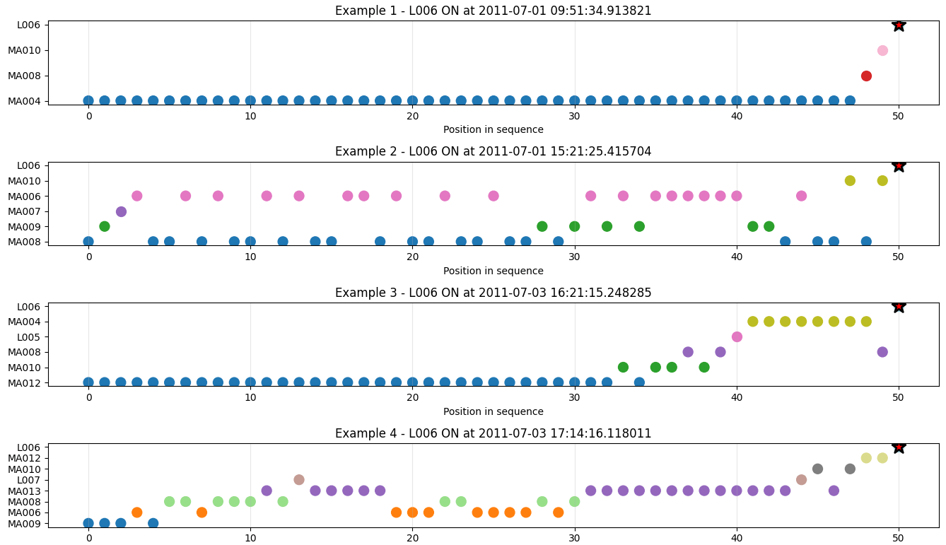
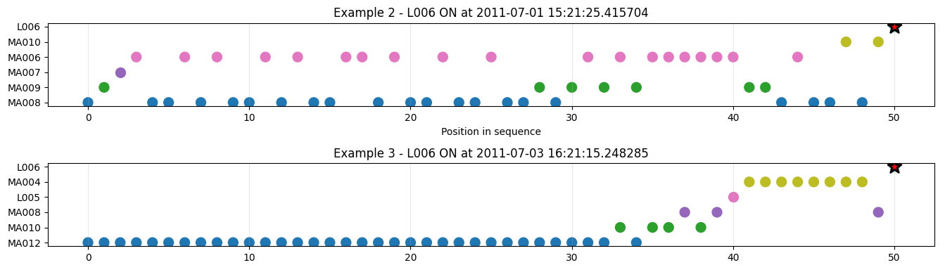
Sample windows
Subset of sensor events in time window of 50.
# DATA EXPLORATION
Dataset Main Problems
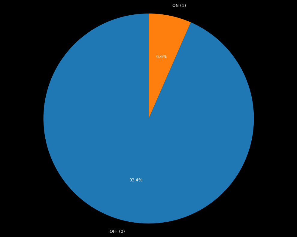
All lights in the dataset are underrepresented compared to other sensors, and the ‘ON’ class is heavily imbalanced with respect to ‘OFF’, with only about 5% of the data related to the switch being actual ON states.
1. Data Imbalance
All motion sensors generate ON signals at every movement interval, producing many records that are often informative but frequently just noise, making pattern extraction more challenging.
2. Noisy Sensors
Data analysis confirmed with high certainty that there are multiple people in the home, making it much more difficult to track individual ‘movements’ and behavior patterns of single occupants.
3. Multiple Humans
# DATA EXPLORATION
- Kitchen main light
- Significant activity (less noise)
- Known to be correlated to daily routines
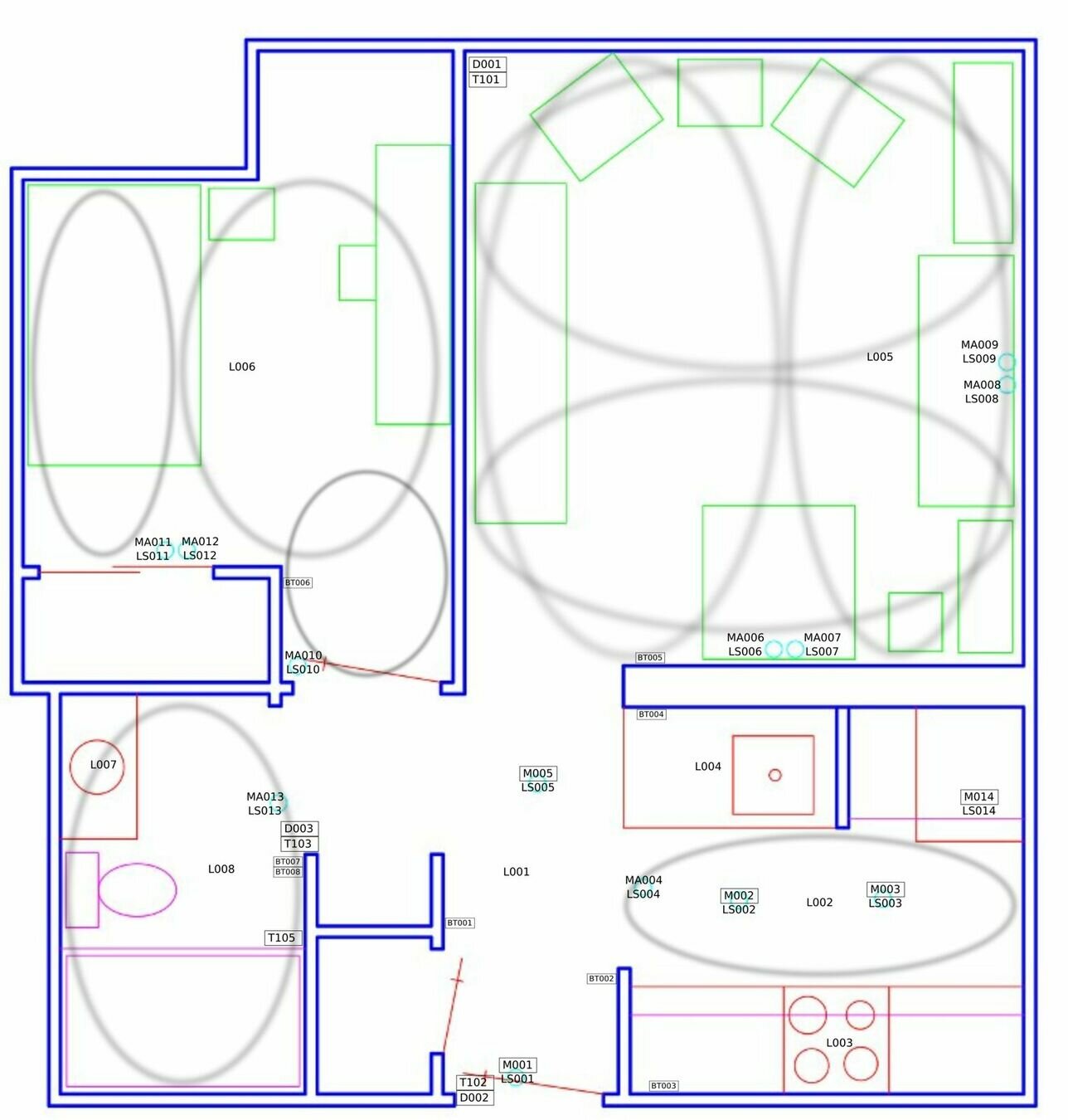
- Home Blueprint key position
- Equilibrate activity presence
Our Target (L002)

Prior
L002 Nowcasting
Feature Engineering and Time Crop
pivot = df_lights.pivot_table(index='Timestamp', columns='Sensor', values='Message', aggfunc='last')

pivot_resampled = pivot.resample('1min').max()
df_lights = pivot_resampled.ffill().bfill()

# ...

df_lights['hour_sin'] = np.sin(2 * np.pi * hour / 24)
df_lights['hour_cos'] = np.cos(2 * np.pi * hour / 24)
df_lights['dow_sin'] = np.sin(2 * np.pi * day_of_week / 7)
df_lights['dow_cos'] = np.cos(2 * np.pi * day_of_week / 7)
df_lights['minute_sin'] = np.sin(2 * np.pi * minute / 60)
df_lights['minute_cos'] = np.cos(2 * np.pi * minute / 60)
df_lights['10min_sin'] = np.sin(2 * np.pi * ((minute // 10) % 6) / 6)
df_lights['10min_cos'] = np.cos(2 * np.pi * ((minute // 10) % 6) / 6)
df_lights['month_sin'] = np.sin(2 * np.pi * month / 12)
df_lights['month_cos'] = np.cos(2 * np.pi * month / 12)

# ...

START_TRAIN_TIMESTAMP = '2011-7-01'
END_TEST_TIMESTAMP = '2013-07-01'
df_lights = df_lights[df_lights.index >= START_TRAIN_TIMESTAMP]
df_lights = df_lights[df_lights.index <= END_TEST_TIMESTAMP]
# PRIOR
Train Objective
target = 'L002'
train_ratio = 0.5
feature_cols = ['hour_sin', 'hour_cos', 'dow_sin', 'dow_cos', 'month_sin', 'month_cos', '10min_sin', '10min_cos'] # 'minute_sin', 'minute_cos']

# PyTorch loss function
loss_cross = nn.BCELoss()

def focal_loss(gamma=2., alpha=0.25):
    """Focal loss for PyTorch"""
    def focal_loss_fixed(y_pred, y_true):
        epsilon = 1e-7
        y_pred = torch.clamp(y_pred, epsilon, 1. - epsilon)

        cross_entropy = -y_true * torch.log(y_pred) - (1 - y_true) * torch.log(1 - y_pred)

        weight = alpha * y_true * torch.pow(1 - y_pred, gamma) + (1 - alpha) * (1 - y_true) * torch.pow(y_pred, gamma)

        loss = weight * cross_entropy

        return torch.mean(torch.sum(loss, dim=-1))

    return focal_loss_fixed

loss_focal = focal_loss(gamma=2., alpha=0.25)
# PRIOR
Train Balancing
class_weights = class_weight.compute_class_weight(
    class_weight='balanced',
    classes=np.unique(y_train),
    y=y_train
)
class_weight_dict = dict(enumerate(class_weights))

print(f"Class weights: {class_weight_dict}")| Class | Weight |
|---|---|
| 0 (Off) | 0.53 |
| 1 (On) | 7.62 |
# PRIOR
MLP & Train
nn1 = build_nn_model(input_shape=(len(X_train.columns), ),
                              output_shape=1,
                              hidden=[128, 128, 64],
                              output_activation='sigmoid',
                              backend='pytorch')

train_nn_model(nn1,
               X_train,
               y_train,
               loss=loss_cross,
               epochs=20,
               verbose=1,
               batch_size=64,
               backend='pytorch',
               class_weight=class_weight_dict)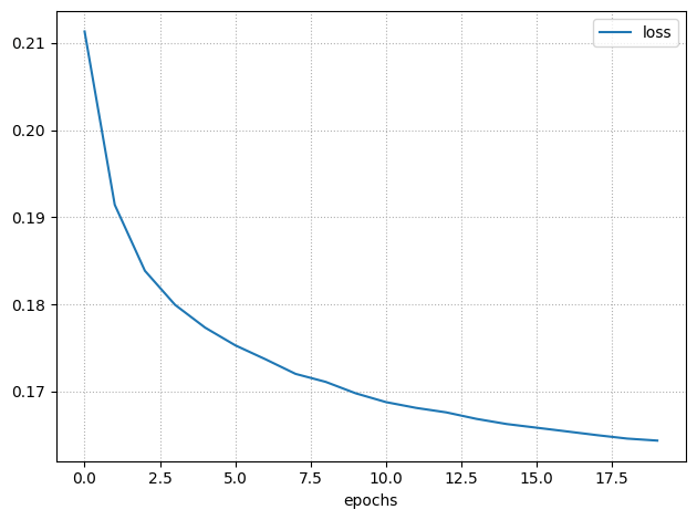
# PRIOR
Results (Overall)
| Class | Precision | Recall | F1-score | Support |
|---|---|---|---|---|
| 0 | 0.97 | 0.91 | 0.94 | 491828 |
| 1 | 0.30 | 0.55 | 0.39 | 34492 |
# PRIOR
Training Set
Test Set
| Class | Precision | Recall | F1-score | Support |
|---|---|---|---|---|
| 0 | 0.94 | 0.88 | 0.91 | 490066 |
| 1 | 0.13 | 0.22 | 0.16 | 36255 |
Results (daytime 8am - 1am)
# PRIOR
Training Set
| Class | Precision | Recall | F1-score | Support |
|---|---|---|---|---|
| 0 | 0.92 | 0.85 | 0.88 | 339270 |
| 1 | 0.14 | 0.24 | 0.17 | 33751 |
Test Set
| Class | Precision | Recall | F1-score | Support |
|---|---|---|---|---|
| 0 | 0.95 | 0.88 | 0.91 | 340038 |
| 1 | 0.30 | 0.54 | 0.39 | 32562 |
Training Set
# PRIOR
Precision-Recall Curves
Test Set
Training Set
# PRIOR
Test Set
Results - One Week
Training Set
# PRIOR
Test Set
Results - Morning
Prior - Limitations
In the following larger models the Prior model demonstrated limited utility as an auxiliary feature due to redundancy with learned temporal representations.
However, it provided crucial value as an interpretable probabilistic baseline for identifying time-of-day bias in light activation patterns, enabling better understanding of household behavior.
# REMARKS
Pattern Mining
Idea
We hypothesized that rule-based mining could provide a baseline for comparison and highlight the most meaningful patterns for light prediction.
Using the Apriori algorithm with metric-based filtering, we extracted a compact ruleset (<40 rules) with strong statistical significance.
# PATTERN MINING
Data structure and Time Crop
START_TIMESTAMP = '2011-7-01'
END_TIMESTAMP = '2011-9-01'
DELTA_SAMPLING = '1s'
# ...
df_pm['Message'] = df_pm['Message'].apply(util_rul.normalize_message)
# ...
for sensor_group, sensor_name in zip(groups, group_names):
  # ...
  df = df[(df['Timestamp'] >= start_timestamp) & (df['Timestamp'] <= end_timestamp)]
  # ...
  pivot = df_group.pivot_table(index='Timestamp', columns='Sensor', values='Message', aggfunc='last')
  # ...
  pivot_resampled = pivot.resample(delta_sampling).max()
  pivot_resampled = pivot_resampled.ffill().bfill()
  pivot_dfs.append(pivot_resampled)
# ...
pivot_df = reduce(lambda left, right: left.join(right, how='outer'), pivot_dfs)
pivot_df = pivot_df.ffill().bfill()

# Keep only rows that are different from the previous row (remove consecutive duplicates)
mask = (df_resampled != df_resampled.shift()).any(axis=1)
df_resampled = df_resampled[mask]
# PATTERN MINING
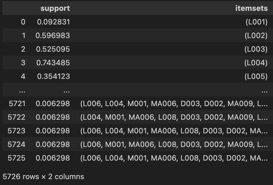
Apriori - Search Item-sets
frequent_itemsets = apriori(df_train,
                            min_support=0.005,
                            use_colnames=True,
                            max_len=10,
                            verbose=1,
                            low_memory=False )
# PATTERN MINING
Itemsets containing L002: 2735
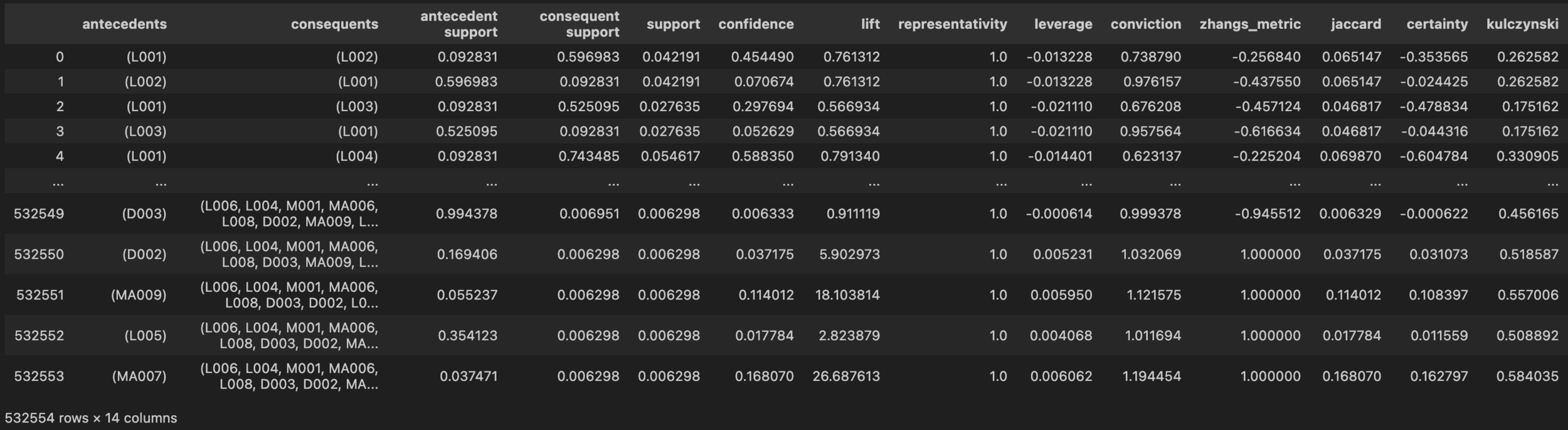
Association rules
rules = association_rules(frequent_itemsets,
                          metric="support",
                          min_threshold=0.005,
                          support_only=False)
# PATTERN MINING
Number of metric-filtered rules predicting L002 ON: 39
Evaluation
# PATTERN MINING
Rules were evaluated by sliding through the dataset and checking if recent events matched any rule with L002 ‘On’ as consequence. Matches yielded positive predictions; non-matches yielded 0.
L005 (Living room - Light)
M005 (Corridor - Motion)
L002 (Kitchen - Light)
Results
| Class | Precision | Recall | F1-score | Support |
|---|---|---|---|---|
| 0 | 0.41 | 1.00 | 0.59 | 35773 |
| 1 | 0.96 | 0.05 | 0.10 | 52990 |
Training Set
Test Set
| Class | Precision | Recall | F1-score | Support |
|---|---|---|---|---|
| 0 | 0.44 | 0.99 | 0.61 | 39188 |
| 1 | 0.54 | 0.01 | 0.02 | 49576 |
# PATTERN MINING
Rules Analysis
# PATTERN MINING
Top Rules (for L002):
- L004, L008, M001 →L002
- L006, L003, L008 →L002
- L007, L003, D002 →L002
High-frequency sensors L005 (living room light) and M005 (corridor motion) demonstrate poor predictive signal-to-noise ratio despite spatial importance, indicating noise sensitivity in rule extraction thresholds.
Forecasting
- RUL prediction
- Light state prediction
- Switch prediction
- Turn on prediction
Task 1
RUL prediction
Idea - RUL Pred.
Predict time until the next light activation with graphical display to users.
Recommend proactive activation when predictions fall within a tunable threshold (e.g., 5 minutes), enabling post-training threshold optimization for practical deployment.
# RUL PREDICTION

Target Creation
target = 'L002'
values = pivot_df_resampled[target].astype(int).values
time_to_on = np.zeros_like(values)

next_on = -1
for i in range(len(values) - 1, -1, -1):
    if values[i] == 1:
        next_on = 0
        time_to_on[i] = 0
    elif next_on == -1:
        time_to_on[i] = 0
    else:
        next_on += 1
        time_to_on[i] = next_on

pivot_df_resampled['time_to_on'] = time_to_on
pivot_df_resampled = pivot_df_resampled[pivot_df_resampled['time_to_on'] < 1000]
MAX_TIME_TO_ON = pivot_df_resampled['time_to_on'].max()
pivot_df_resampled['time_to_on'] = pivot_df_resampled['time_to_on'] / MAX_TIME_TO_ON
# RUL PREDICTION
Regression Tree
# Regression tree
reg = DecisionTreeRegressor(max_depth=8, random_state=42)
reg.fit(X_train, y_train)

# Predict
y_pred = reg.predict(X_test)
# RUL PREDICTION
# Filter the values of y_test where the ground truth is between 1 and 6
mask = (y_test*MAX_TIME_TO_ON >= 1) & (y_test*MAX_TIME_TO_ON <= 6)
y_test_filtered = y_test[mask]*MAX_TIME_TO_ON
y_pred_filtered = y_pred[mask]*MAX_TIME_TO_ON

mae_filtered = mean_absolute_error(y_test_filtered, y_pred_filtered)
r2_filtered = r2_score(y_test_filtered, y_pred_filtered)
MAE: 93.2
R2: 0.50
MAE: 88.9
R2: 0.22
Original
Filtered (max 6min before)
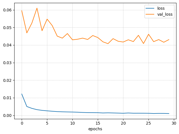
MLP & Train
nn2 = util_rul.build_nn_model(input_shape=(len(X_train.columns), ),
                              output_shape=1,
                              hidden=[32, 32])

history = util_rul.train_nn_model(nn2,
                                  X_train,
                                  y_train,
                                  validation_split=0.2,
                                  loss='mse',
                                  epochs=30,
                                  batch_size=32,
                                  verbose=1)
# RUL PREDICTION
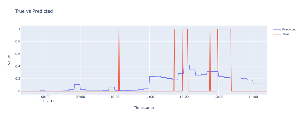
[ MLP ] Prediction-Target Plot
# RUL PREDICTION
Text
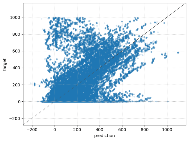
[ MLP ] Results on Test set
# RUL PREDICTION
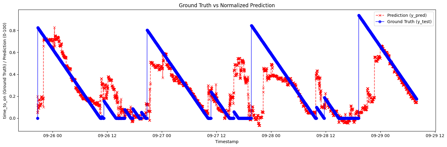
RUL - Limitations
# RUL PREDICTION
- The RUL model demonstrates strong nocturnal pattern learning, achieving good precision from night to morning, but exhibits poor daytime performance with substantial false positives.
- The fundamental challenge stems from high intra-day variability: activations occur in rapid succession or hours apart.
Task 2
Light state prediction
Idea - State Pred.
Predict which state the light will be in during the next successive time unit.
The idea was to learn which ‘activities’ in the home the light state was associated with, and exploit this to understand when it should be on and when it should be off, by modeling the light state throughout the entire time range.
Predicted probabilities above a threshold could serve as a continuous control signal for adaptive light dimming levels.
# LIGHT STATE PREDICTION
0%
100%
50%
Sequence Creation
DELTA_SAMPLING = '1min'
DELTA_FORECAST = 1
# ...
df['Message'] = df['Message'].apply(util_rul.normalize_message)
# ...
START_TRAIN_TIMESTAMP = '2011-7-01'
END_TEST_TIMESTAMP = '2013-07-01'
df_lights = df_lights[df_lights.index >= START_TRAIN_TIMESTAMP]
df_lights = df_lights[df_lights.index <= END_TEST_TIMESTAMP]
# ...

def create_sequences(X, y, n_timesteps=4):
    Xs, ys = [], []
    for i in tqdm(range(len(X) - n_timesteps + 1)):
        Xs.append(X[i:i+n_timesteps])
        ys.append(y[i+n_timesteps-1])
    return np.array(Xs), np.array(ys)

# Create LSTM sequences
X_train_lstm, y_train_lstm = create_sequences(X_train.values,
                                              y_train.values,
                                              n_timesteps=n_timesteps)
X_test_lstm, y_test_lstm = create_sequences(X_test.values,
                                            y_test.values,
                                            n_timesteps=n_timesteps)
# LIGHT STATE PREDICTION
Class Weight
class_weights = class_weight.compute_class_weight(
    'balanced',
    classes=np.unique(y_train_lstm),
    y=y_train_lstm
)
class_weight_dict = {i: class_weights[i] for i in range(len(class_weights))}
# LIGHT STATE PREDICTION
| Class | Weight |
|---|---|
| 0 (Off) | 0.71 |
| 1 (On) | 1.68 |
Model - LSTM
model = Sequential([
    Input(shape=(X_train_lstm.shape[1], X_train_lstm.shape[2])),
    LSTM(256),
    Dense(64, activation='relu'),
    Dense(1, activation='sigmoid')
])

loss_cross = keras.losses.BinaryFocalCrossentropy(
    apply_class_balancing=False,
    alpha=0.25,
    gamma=2.0,
    from_logits=False,
    label_smoothing=0.1,
    axis=-1,
    reduction="sum_over_batch_size",
    name="binary_focal_crossentropy",
    dtype=None,
)

opt = keras.optimizers.Adam(learning_rate=0.001)

model.compile(optimizer=opt, loss=loss_cross)
# LIGHT STATE PREDICTION
Train
history = model.fit(
    X_train_lstm, y_train_lstm,
    epochs=10,
    batch_size=256,
    validation_data=(X_test_lstm, y_test_lstm),
    verbose=1,
    shuffle=True,
    class_weight=class_weight_dict
)
# LIGHT STATE PREDICTION
Results
| Class | Precision | Recall | F1-score | Support |
|---|---|---|---|---|
| 0 | 0.97 | 1.00 | 0.99 | 369874 |
| 1 | 0.99 | 0.94 | 0.97 | 156436 |
Training Set
Test Set
# LIGHT STATE PREDICTION
| Class | Precision | Recall | F1-score | Support |
|---|---|---|---|---|
| 0 | 0.98 | 1.00 | 0.99 | 395476 |
| 1 | 0.99 | 0.93 | 0.96 | 130835 |
But... All that glitters is not gold
Task formulation induces exploitable shortcut through label stationarity bias.
Post-transition, model predicts prior stable state rather than forecasting upcoming transitions.
State transition events constitute minority class relative to stationary periods, creating severe imbalance that rewards conservative predictions and penalizes transition detection.
# LIGHT STATE PREDICTION
Cost Model - Limitations
- Initially we defined a cost model that evaluates predictions based on temporal proximity to actual events within a defined window, weighting more predictions closer to events.
-
But, defining the cost model is inherently difficult:
- What window is acceptable? (1 min or 1 hour?)
- How to weight different temporal distances?
- How to account for data preprocessing?
- Multiple interdependent design choices lack clear optimal answers, making generalization among tasks challenging.
# REMARKS
Task 3
Switch prediction
Idea - Switch Pred.
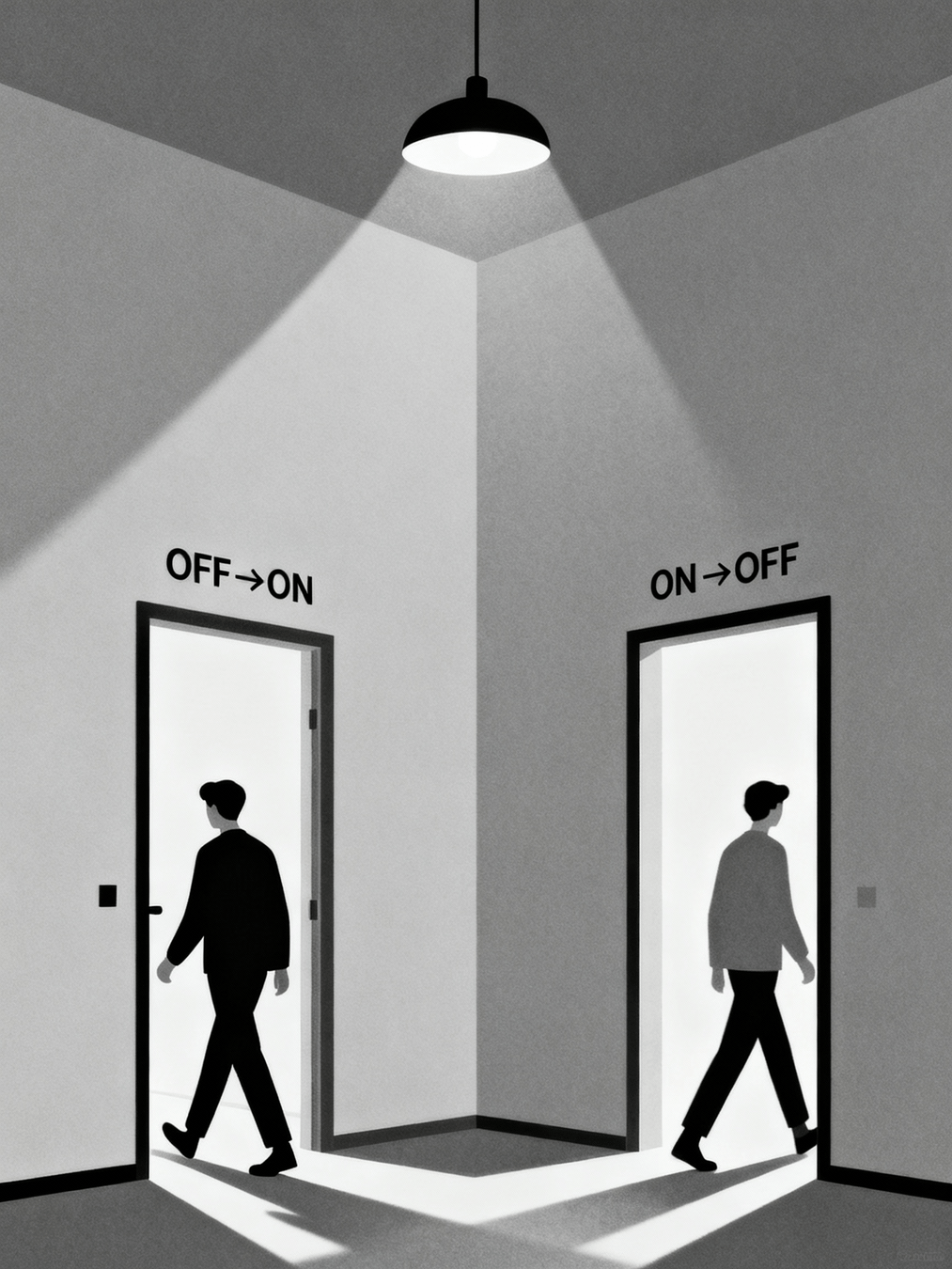
Develop a binary classification model for switch event prediction at t+1, identifying state transitions (OFF→ON or ON→OFF) as distinct from no-switch time steps.
Captures transition dynamics separately from state maintenance patterns.
# SWITCH PREDICTION
Sequence Creation
start_timestamp = '2011-7-01'
end_timestamp = '2013-07-01'

DELTA_SAMPLING = '1min'
DELTA_FORECAST = 1

# ...

# Create switch target: 1 only at transitions (0->1 or 1->0)
pivot_df_resampled[TARGET] = pivot_df_resampled['L002'].diff().abs().fillna(0)
# SWITCH PREDICTION
State Sequence LSTM
model = Sequential([
    Input(shape=(X_train_lstm.shape[1], X_train_lstm.shape[2])),
    LSTM(256),
    Dense(64, activation='relu'),
    Dense(1, activation='sigmoid')
])

loss_cross = keras.losses.BinaryFocalCrossentropy(
    apply_class_balancing=False,
    alpha=0.25,
    gamma=2.0,
    from_logits=False,
    label_smoothing=0.1,
    axis=-1,
    reduction="sum_over_batch_size",
    name="binary_focal_crossentropy",
    dtype=None,
)

opt = keras.optimizers.Adam(learning_rate=0.001)

model.compile(optimizer=opt, loss=loss_cross)
# SWITCH PREDICTION
Weight Balancing
class_weights = class_weight.compute_class_weight(
    'balanced',
    classes=np.unique(y_train_lstm),
    y=y_train_lstm
)
class_weight_dict = {i: class_weights[i] for i in range(len(class_weights))}
# SWITCH PREDICTION
| Class | Weight |
|---|---|
| 0 (Off) | 0.5 |
| 1 (On) | 110.9 |
Train
history = model.fit(
    X_train_lstm, y_train_lstm,
    epochs=10,
    batch_size=256,
    validation_data=(X_test_lstm, y_test_lstm),
    verbose=1,
    shuffle=True,
    class_weight=class_weight_dict
)
# SWITCH PREDICTION
Results
| Class | Precision | Recall | F1-score | Support |
|---|---|---|---|---|
| 0 | 1.00 | 1.00 | 1.00 | 523937 |
| 1 | 0.27 | 0.02 | 0.04 | 2373 |
Training Set
Test Set
| Class | Precision | Recall | F1-score | Support |
|---|---|---|---|---|
| 0 | 1.00 | 1.00 | 1.00 | 523891 |
| 1 | 0.14 | 0.01 | 0.02 | 2420 |
# SWITCH PREDICTION
Limitations
# SWITCH PREDICTION
We observed that the task remained overly complex: the model had to simultaneously learn discriminative patterns for both OFF→ON and ON→OFF transitions.
To address this, we made the strategic decision to further simplify the task by focusing exclusively on turn-on prediction.
Task 4
Turn on prediction
Idea - Turn on Pred.
Simplify the prediction task by focusing exclusively on turn-ON events (OFF→ON).
Hypothesize that activation-preceding patterns are more discriminative than general background patterns, improving classifier performance.
# TURN ON PREDICTION

[State] Sequence Creation
start_timestamp = '2011-7-01'
end_timestamp = '2013-07-01'

DELTA_SAMPLING = '1min'
DELTA_FORECAST = 1

# ...

# Create on_only target: 1 only at 0->1 transitions (light turning ON)
pivot_df_resampled[TARGET] = ((pivot_df_resampled['L002'].diff() == 1).astype(int))
# TURN ON PREDICTION
Difference from Switch Predition
State Sequence LSTM
model = Sequential([
    Input(shape=(X_train_lstm.shape[1], X_train_lstm.shape[2])),
    LSTM(256),
    Dense(64, activation='relu'),
    Dense(1, activation='sigmoid')
])

loss_cross = keras.losses.BinaryFocalCrossentropy(
    apply_class_balancing=False,
    alpha=0.25,
    gamma=2.0,
    from_logits=False,
    label_smoothing=0.1,
    axis=-1,
    reduction="sum_over_batch_size",
    name="binary_focal_crossentropy",
    dtype=None,
)

opt = keras.optimizers.Adam(learning_rate=0.001)

model.compile(optimizer=opt, loss=loss_cross)
# TURN ON PREDICTION
Weight Balancing
class_weights = class_weight.compute_class_weight(
    'balanced',
    classes=np.unique(y_train_lstm),
    y=y_train_lstm
)
class_weight_dict = {i: class_weights[i] for i in range(len(class_weights))}| Class | Weight |
|---|---|
| 0 (Off) | 0.5 |
| 1 (On) | 221.9* |
# TURN ON PREDICTION
* double respect to Switch pred. task
Results
| Class | Precision | Recall | F1-score | Support |
|---|---|---|---|---|
| 0 | 1.00 | 1.00 | 1.00 | 525129 |
| 1 | 0.18 | 0.22 | 0.19 | 1186 |
Training Set
Test Set
| Class | Precision | Recall | F1-score | Support |
|---|---|---|---|---|
| 0 | 1.00 | 1.00 | 1.00 | 526316 |
| 1 | 0.05 | 0.11 | 0.07 | 1210 |
# TURN ON PREDICTION
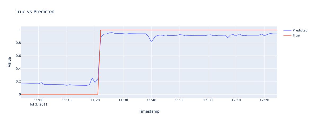
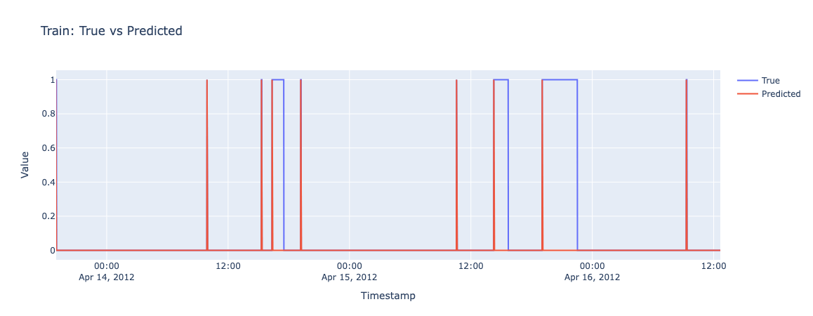
Results on Test set Analysis
# TURN ON PREDICTION
Pred: 9.24🟢
GT: 9.35
Pred: 8.29
GT: 9.35
🟡
Pred: 9.02🟢
GT: 9.15
Pred: 8:30🟡
GT: 9:37
Pred: 7:50🟡
GT: 9:05
GT: 9:40🟠
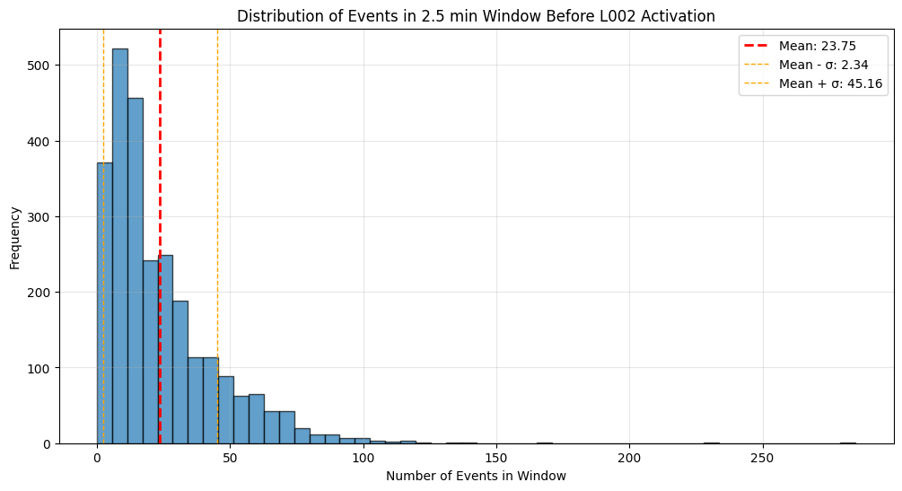
[State seq. Turn On] Cost Model
# TURN ON PREDICTION
| Segments | Number | Mean (length) | Sigma (length) | % of total events |
|---|---|---|---|---|
| Correct | 123 | 2.13 | 1.62 | 10% |
| Wrong | 365 | 2.49 | 2.81 | 28% |
| Tot: 488 |
Cost model evaluated on 1260 "Turn-On" events:
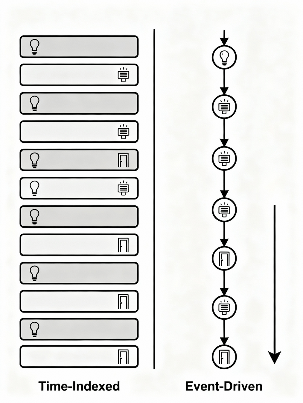
Idea - Event Seq.
- Fundamental paradigm shift: rather than maintaining home state as temporal rows, we structure data using individual events as rows.
- This transforms the representation from a time-aligned state sequence (with concurrent events within each time unit) to an event-centric sequence of successive occurrences.
- Correspondingly, inference changes from fixed-interval (per time unit) to event-triggered: predictions occur whenever an event happens, not at regular time intervals.
# TURN ON PREDICTION
[Event] Sequence Creation
sequence_length = 50
embedding_dim = 32
PRED_FORWARD = 2  # minutes
PRED_FORWARD_SECONDS = 30  # seconds

# ...

df_event_log = df_event_log.sort_values("Timestamp").reset_index(drop=True)
df_event_log["event"] = df_event_log["Sensor"].astype(str) + "_" + df_event_log["Message"].astype(str)

unique_events = df_event_log["event"].unique()
# +1 to reserve 0 for padding
event_to_idx = {event: idx + 1 for idx, event in enumerate(unique_events)}
idx_to_event = {idx: event for event, idx in event_to_idx.items()}
# +1 for padding
num_events = len(event_to_idx) + 1
# TURN ON PREDICTION
LSTM - Without Time Embedding
class LSTMModel(nn.Module):
    def __init__(self, num_events, embedding_dim, hidden_dim=64, num_layers=2, dropout=0.3):
        super(LSTMModel, self).__init__()
        self.embedding = nn.Embedding(num_events, embedding_dim, padding_idx=0)
        self.lstm = nn.LSTM(embedding_dim, hidden_dim, num_layers,
                           batch_first=True, dropout=dropout if num_layers > 1 else 0)
        self.dropout = nn.Dropout(dropout)
        self.fc1 = nn.Linear(hidden_dim, 16)
        self.fc2 = nn.Linear(16, 1)
        self.relu = nn.ReLU()
        self.sigmoid = nn.Sigmoid()

    def forward(self, x):
        embedded = self.embedding(x)
        lstm_out, (h_n, c_n) = self.lstm(embedded)
        # Use last hidden state
        last_hidden = h_n[-1]
        out = self.dropout(last_hidden)
        out = self.relu(self.fc1(out))
        out = self.dropout(out)
        out = self.sigmoid(self.fc2(out))
        return out
# TURN ON PREDICTION
Class Weight
class_weight_dict = util_rul.get_class_weights(dataset_train)
pos_weight = torch.tensor([class_weight_dict[1] / class_weight_dict[0]]).to(device)

# ...

criterion = nn.BCEWithLogitsLoss(pos_weight=pos_weight)
# TURN ON PREDICTION
| Class | Weight |
|---|---|
| 0 (Off) | 0.5 |
| 1 (On) | 20.1 |
Results
| Class | Precision | Recall | F1-score | Support |
|---|---|---|---|---|
| 0 | 0.99 | 0.84 | 0.91 | 1528454 |
| 1 | 0.09 | 0.65 | 0.16 | 39082 |
Training Set
Test Set
| Class | Precision | Recall | F1-score | Support |
|---|---|---|---|---|
| 0 | 0.98 | 0.84 | 0.90 | 1525122 |
| 1 | 0.08 | 0.53 | 0.14 | 42414 |
# TURN ON PREDICTION
Handling imbalanced and noisy data
# TURN ON PREDICTION
Balancing Strategy
Objective: Create a dataset with a more balanced positive/negative ratio while maintaining data diversity.
- Partitions samples into positive/negative groups, then creates a balanced dataset by oversampling positives and undersampling negatives to achieve a target ratio. Combines both groups and shuffles to avoid ordering bias.
Denoising Strategy
Problem: Consecutive identical sensor events create redundancy (e.g., 10× same sensor spike)
- Solution: Identifies consecutive runs of identical sensors and compresses series exceeding max consecutive event repeats by keeping first/last events plus uniformly-sampled intermediates. Preserves temporal structure while reducing noise from sensor jitter.
Results Test set - Model Variants
Without Time embedding (previous result)
With Time embedding + Balancing + Denoising
| Class | Precision | Recall | F1-score | Support |
|---|---|---|---|---|
| 0 | 0.97 | 1.00 | 0.99 | 1525122 |
| 1 | 0.42 | 0.03 | 0.05 | 42414 |
# TURN ON PREDICTION
With Time embedding
| Class | Precision | Recall | F1-score | Support |
|---|---|---|---|---|
| 0 | 0.98 | 0.97 | 0.98 | 1525122 |
| 1 | 0.18 | 0.21 | 0.19 | 42414 |
| Class | Precision | Recall | F1-score | Support |
|---|---|---|---|---|
| 0 | 0.98 | 0.84 | 0.90 | 1525122 |
| 1 | 0.08 | 0.53 | 0.14 | 42414 |
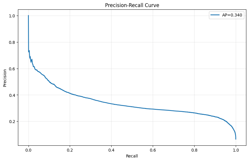
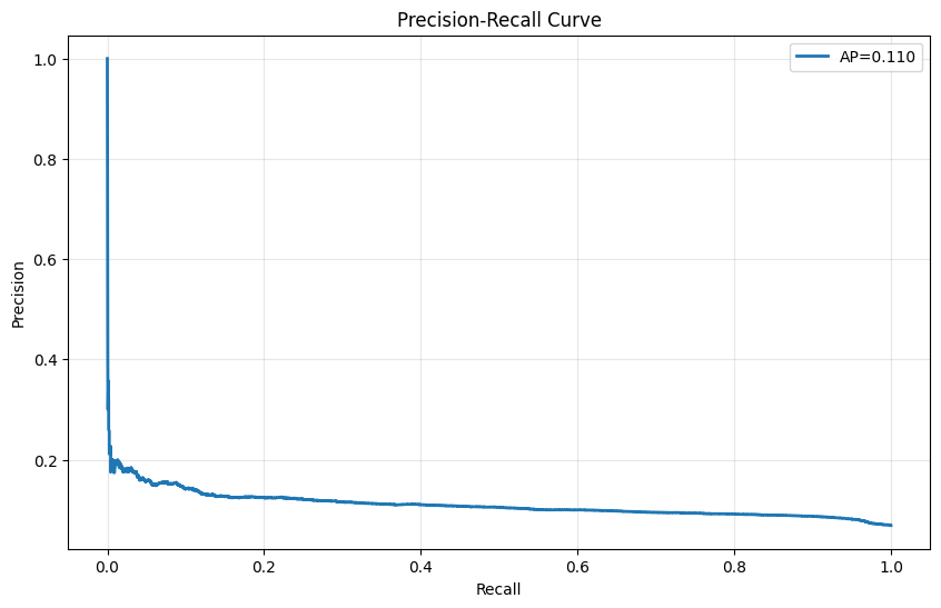
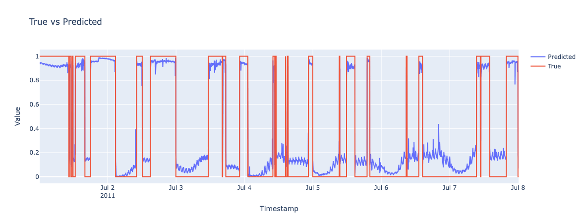
Why this Precision-Recall is Good
With Time embedding + Balancing + Denoising
| Class | Precision | Recall | F1-score | Support |
|---|---|---|---|---|
| 0 | 0.97 | 1.00 | 0.99 | 1525122 |
| 1 | 0.42 | 0.03 | 0.05 | 42414 |
# TURN ON PREDICTION
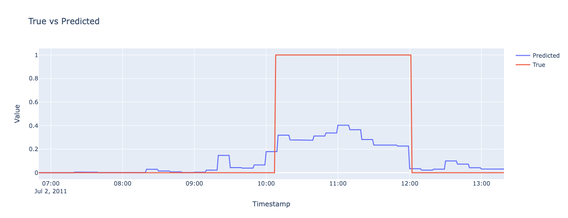
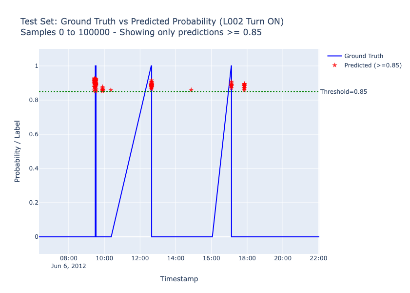
Daily habits that are stable (e.g. morning kitchen light) yield good metrics.
However, many daily activations show heterogeneous inter-day patterns with irregular, unstable dependencies difficult to model.
Strategic choice: ~8 higher-precision predictions daily
(~3.5 correct) rather than many low-confidence predictions.
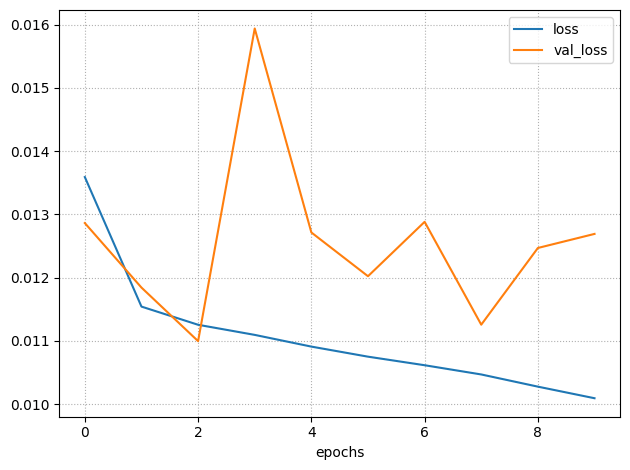
Analysis and Limitations
# TURN ON PREDICTION
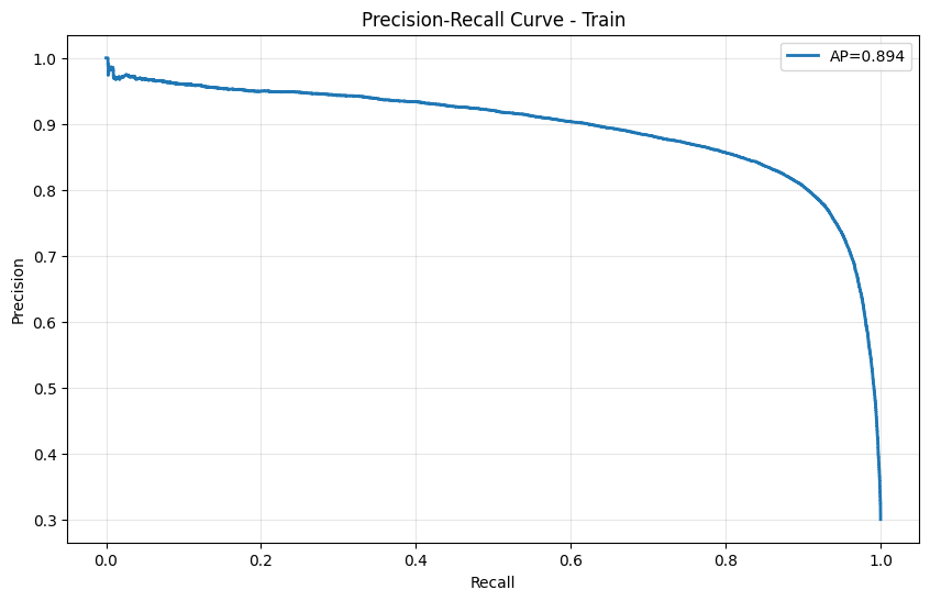
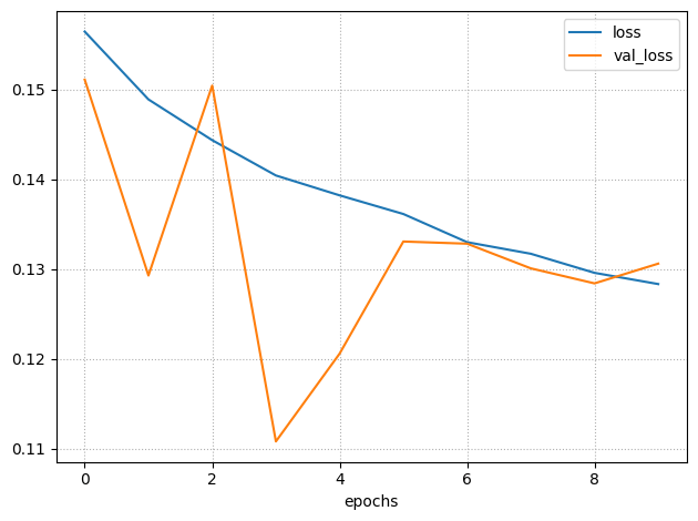
- The training Precision-Recall curve exhibits strong performance (AP=0.894), indicating a tendency toward overfitting.
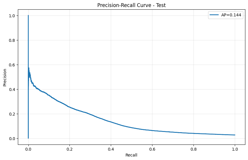
- However, the test Precision-Recall curve reveals significant performance degradation (AP=0.144), showing that high precision is maintained only on a very limited number of samples.
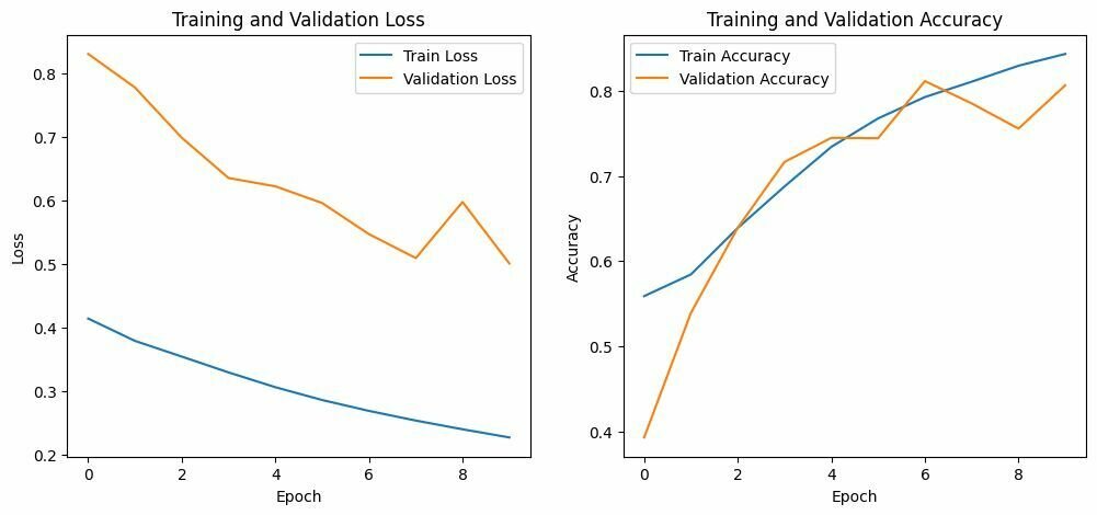
- The delicate training dynamics observed across epochs stem directly from the original data imbalance and noise, creating optimization challenges.
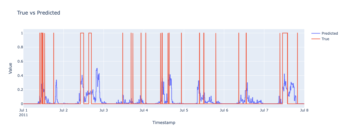
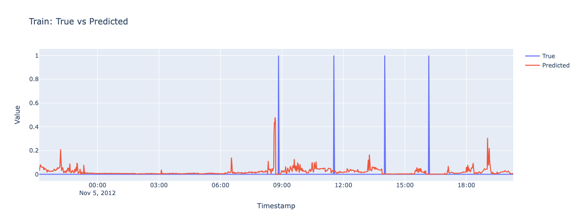
Results on Test set
# TURN ON PREDICTION
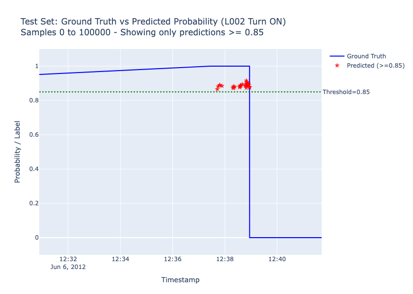
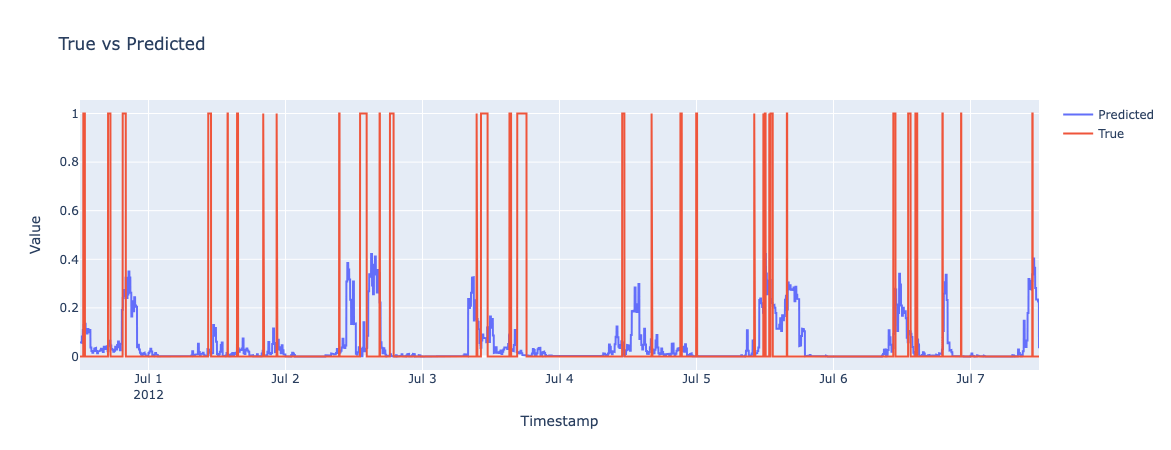
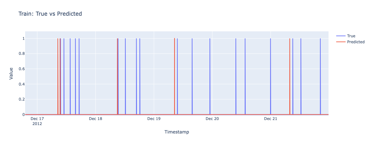
Results on Test set
# TURN ON PREDICTION
Deploy-oriented Tests
# TURN ON PREDICTION
Temporal adaptation (monthly fine-tuning):
- Address distribution shift via incremental retraining on recent data to capture evolving behavioral patterns.
Multi-task learning (multi-label model):
- Joint prediction across all lights leveraging inter-light dependencies rather than independent single-light classifiers for improved whole-home coverage.
But... both strategies require deployment considerations for production-grade performance parity with single-light validation.
{The End}
Thank you for the attention!
Code
By alessandro sciarrillo
