Maxout Networks
ICML'13
Ian J. Goodfellow - David Warde-Farley - Mehdi Mirza - Aaron Courville - Yoshua Bengio

Café de la Recherche #1 @Sicara
3 mai 2018 - Antoine Toubhans


Abstract
We consider the problem of designing models to leverage a recently introduced approximate model averaging technique called dropout. We define a simple new model called maxout (so named because its output is the max of a set of inputs, and because it is a natural companion to dropout) designed to both facilitate optimization by dropout and improve the accuracy of dropout’s fast approximate model averaging technique. We empirically verify that the model successfully accomplishes both of these tasks. We use maxout and dropout to demonstrate state of the art classification performance on four benchmark datasets: MNIST, CIFAR-10, CIFAR100, and SVHN.
A regularization technique for NN
The paper's thesis
Benchmarks
Maxout Networks
- Introduction
- Review of dropout
-
Description of
maxout -
Maxout is a universal approximator - Benchmark results
- Comparison to rectifiers
- Model averaging
- Optimization
- Conclusion
Maxout Networks
- Introduction
- Review of dropout
- Description of maxout
- Maxout is a universal approximator
- Benchmark results
- Comparison to rectifiers
- Model averaging
- Optimization
- Conclusion
Maxout Networks
- Introduction
- Review of dropout
- Description of maxout
- Maxout is a universal approximator
- Benchmark results
- Comparison to rectifiers
- Model averaging
- Optimization
- Conclusion
Dropout: a bagging technique
Dropout training is similar to bagging. [2]
[2] Breiman, Leo. Bagging predictors. Machine Learning, 24 (2):123–140, 1994
BAGGING = Bootstrap AGGregatING
Train different models on different subsets of the data
e.g. random forest is bagging of decision trees
Bagging overview
\mathbb{E}\left[\left(\frac{1}{N}\sum_i\varepsilon_i\right)^2\right]
=
\frac{1}{N^2} \mathbb{E}\left[
\sum_i \varepsilon_i^2 + \sum_{i \neq j}\varepsilon_i\varepsilon_j
\right]
- a regularization technique
- key idea: different models will not make the same errors on the test set
=
\frac{1}{N} V
+
\frac{N-1}{N} C
\mathbb{E}\left[\varepsilon_i\right] = 0
\quad
V = \mathbb{E}\left[\varepsilon_i^2\right]
\quad
C = \mathbb{E}\left[\varepsilon_i\varepsilon_j\right]
Error of the i-th model on the test set:
\varepsilon_i

Dropout overview
Approximation of bagging an exponentially large number of neural networks.
- the sub-models share parameters
- approximated inference (weight scaling inference rule)
Dropout overview

Training an ensemble of NN


For each training example:
- randomly sample a mask
- the probability of each entry being 1 is a hyperparameter
- stochastic training
- feedforward and
backprop as usual
p(y\vert x; \theta)
\mu
p(y\vert x;\theta,\mu)
Dropout inference
p(y\vert x;\theta)
=
\sum_\mu p(\mu) p(y\vert x;\theta,\mu)
Arithmetic mean:
Untractable!

Dropout inference
\hat{p}(y\vert x;\theta)
=
\Pi_\mu p(y\vert x;\theta,\mu)^{p(\mu)}
Geometic mean:
The trick: use geometric mean instead
p(y\vert x;W, b,\mu) = \text{softmax}(W^T(x \circ \mu)+b)_y
If
Then
p(y\vert x;W,b)
=
\text{softmax}(\frac{1}{2}W^Tx+b)_y
Approximations:
- Geometric mean vs arithmetic mean
- Theoretical proof for one layer only
the weight scaling rule
works well empirically
Dropout inference - Sketch of proof
p(\mu) = \frac{1}{2^d}
\propto \left( \Pi_\mu \text{softmax}(W^T(x \circ \mu)+b)_y \right) ^{2^{-d}}
p(y\vert x;W,b)
\propto
\Pi_\mu p(y\vert x;W,b,\mu)^{p(\mu)}
\text{softmax}(z)_y = \frac{e^{z_y}}{\sum_{y'}e^{z_{y'}}}
\propto \left( \Pi_\mu \text{exp}(W^T(x \circ \mu)+b)_y \right) ^{2^{-d}}
\propto \text{exp} \left( 2^{-d} \sum_\mu (W^T(x \circ \mu)+b)_y \right)
\propto \text{exp} \left( \frac{1}{2} (W^Tx+b )_y \right)
= \text{softmax} \left( \frac{1}{2} (W^Tx+b ) \right)_y
Maxout Networks
- Introduction
- Review of dropout
- Description of maxout
- Maxout is a universal approximator
- Benchmark results
- Comparison to rectifiers
- Model averaging
- Optimization
- Conclusion
"
Maxout units: a generalization of ReLU
[2] Deep Learning Book, p188.
"The maxout model is simply a feed-forward architecture[...] that uses a new type of activation function: the maxout unit." [1]
[1] ICML'13, Maxout networks, Goodfellow and Al.
Maxout units: a generalization of ReLU
\text{ReLU}(z) = \text{max}(0, z)

How to compare activation functions:
- saturation
- piecewise linear
- bounded
- sparse activation [3]
[3] Deep Sparse Rectifier Neural Networks, Bengio and Al.
x \in \mathbb{R}^d, \quad W \in \mathbb{R}^{d \times m}, \quad b \in \mathbb{R}^m
Hidden Layer + ReLU
y = \text{ReLU}\left( W^Tx + b \right) \in \mathbb{R}^m
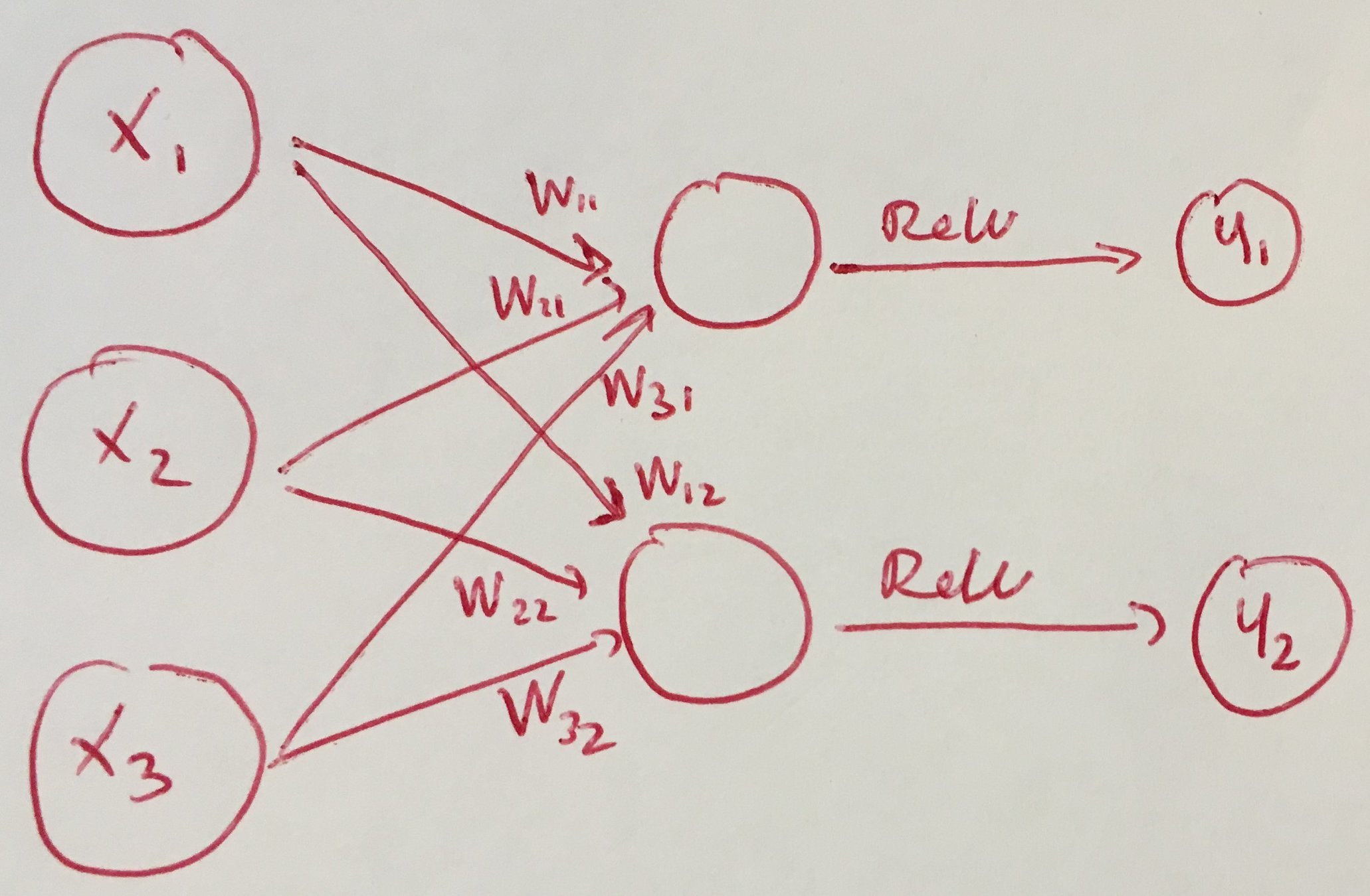
Maxout definition
z = x^TW + b \in \mathbb{R}^{m \times k}
\quad
y_i = \text{max}_{j\in[1, k]}(z_{ij})
x \in \mathbb{R}^d, \quad W \in \mathbb{R}^{d \times m \times k}, \quad b \in \mathbb{R}^{m \times k}
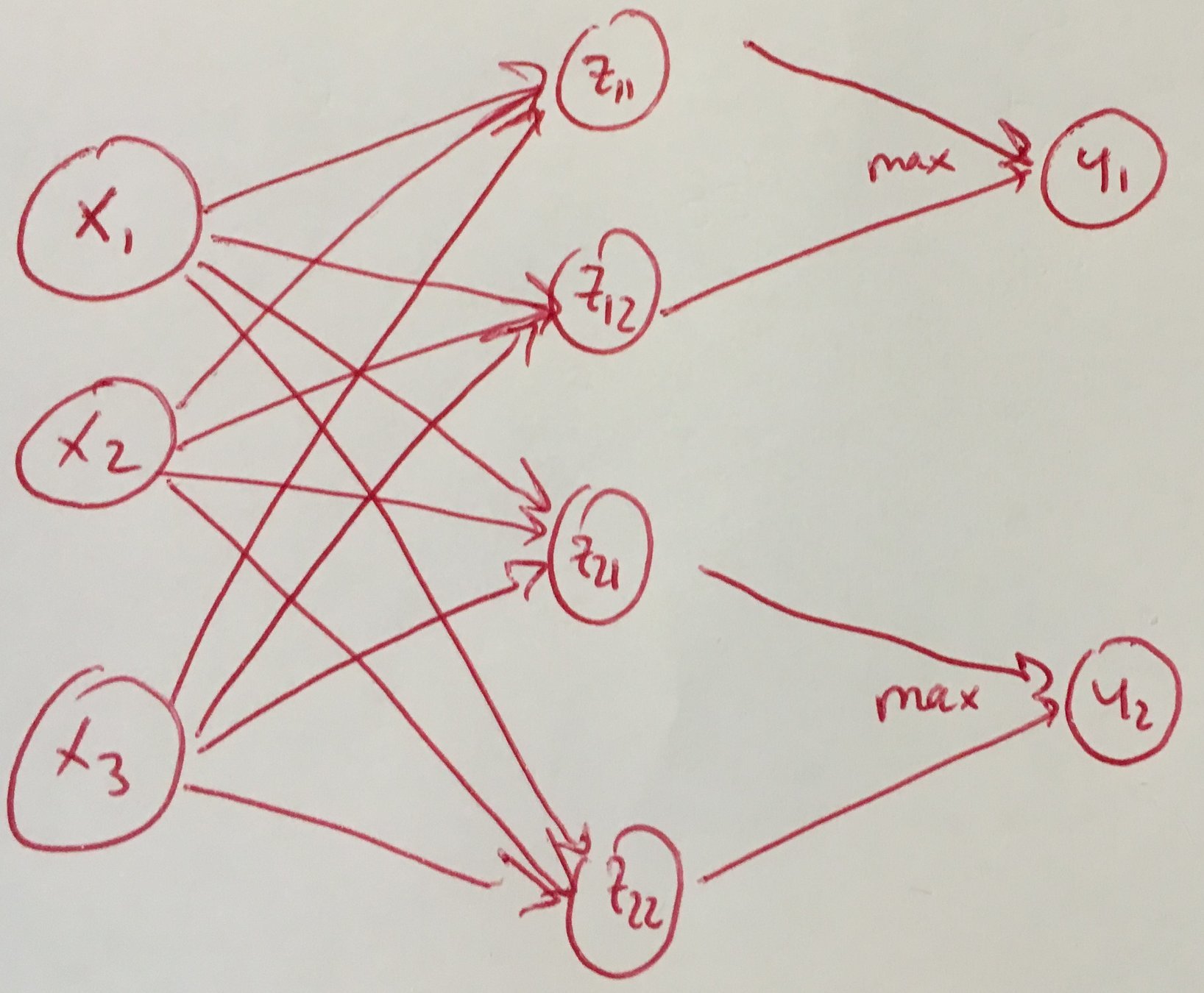
Maxout definition

Maxout for CNN
In a convolutional network, a maxout feature map can be constructed by taking the maximum across k affine feature maps (i.e., pool across channels, in addition spatial locations).
Maxout Max-pooling !
\neq
- (2D) Max-pooling: only across spatial dimensions
- Maxout: across all dimension (channels and spacial)
Channel pooling
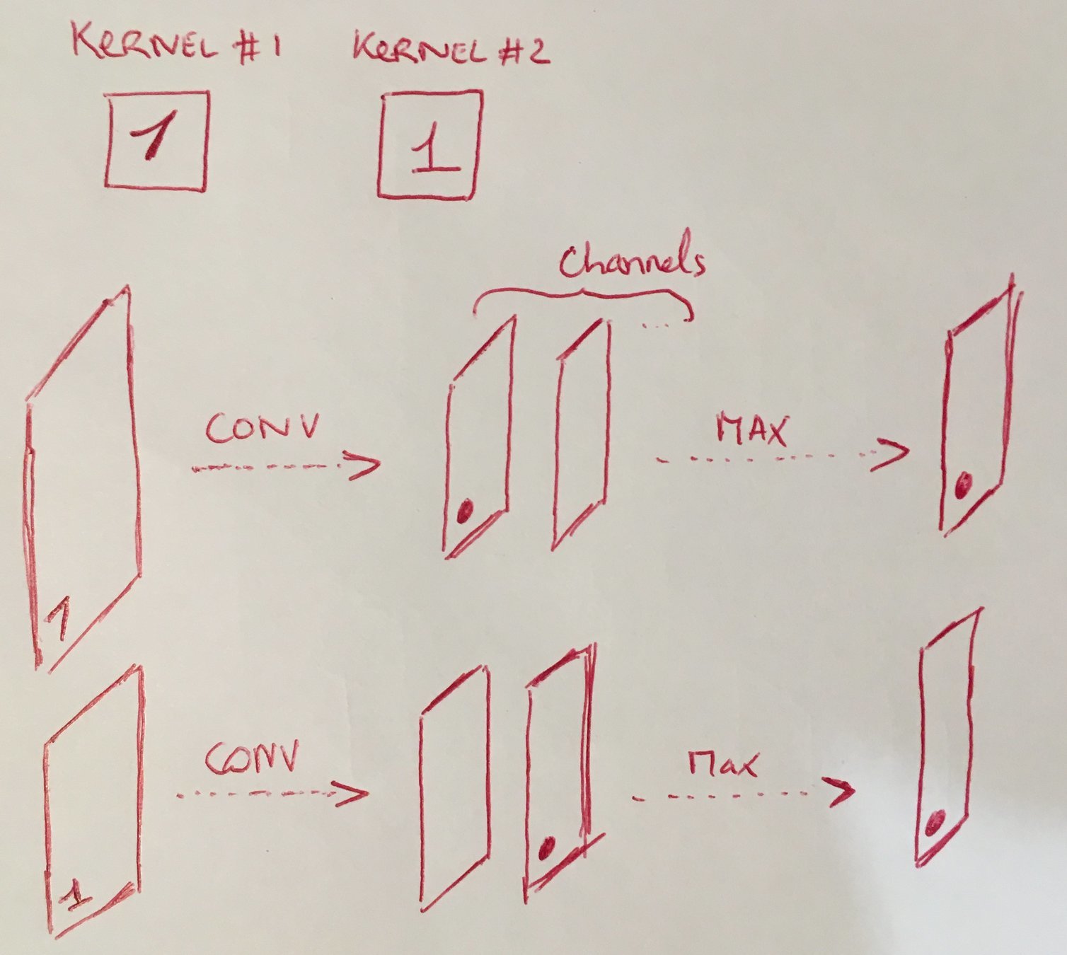
Maxout for CNN

Maxout Networks
- Introduction
- Review of dropout
- Description of maxout
- Maxout is a universal approximator
- Benchmark results
- Comparison to rectifiers
- Model averaging
- Optimization
- Conclusion
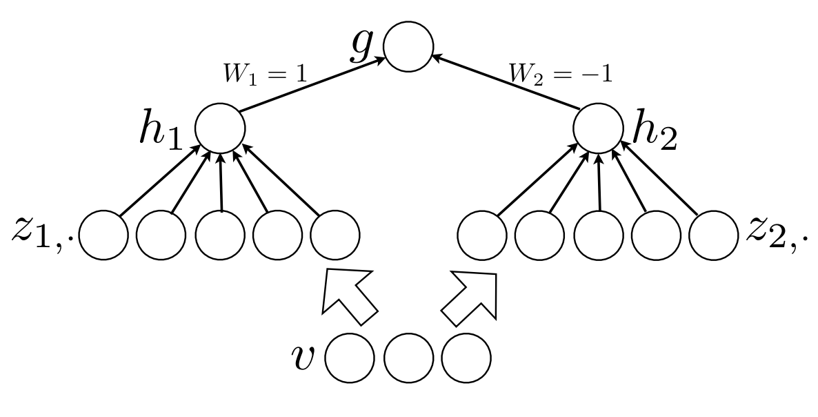
A Universal Approximator
Any feedforward NN with one hidden layer with any "squashing" activation function and a linear out is a universal approximator [5]
[5] Multilayer feedforward networks are universal approximators, Hornik and Al., 1989
One-layer perceptron can not represent the Xor function [4]
[4] Minsky and Papert, 1969
*
(*) provided sufficiently many hidden units are available

A Universal Approximator

Sketch of proof


Sketch of proof
Maxout Networks
- Introduction
- Review of dropout
- Description of maxout
- Maxout is a universal approximator
- Benchmark results
- Comparison to rectifiers
- Model averaging
- Optimization
- Conclusion
Benchmark results
MNIST
60000 x 28 x 28 x 1
10 classes
4 datasets, comparison to the state of the art (2013)
CIFAR-10
60000 x 32 x 32 x 3
10 classes
CIFAR-100
60000 x 32 x 32 x 3
100 classes
SVHN
>600K x 32 x 32 x 3
Identify digits in the images
Benchmark results - MNIST

The permutation invariant version:
- should be unaware of the 2D structure, meaning no convolution
- 2 dense Maxout layers + softmax
- dropout regularization
- best result without the use of unsupervised pretraining.
Benchmark results - MNIST
The CNN version:
- 3 convolutional maxout layers + 1 dense layer + softmax

Benchmark results
- Other results in the paper
- Dropout + Maxout achieve state of the art performance
Maxout Networks
- Introduction
- Review of dropout
- Description of maxout
- Maxout is a universal approximator
- Benchmark results
- Comparison to rectifiers
- Model averaging
- Optimization
- Conclusion
Comparison to rectifiers
Why are the results better?
- improved preprocessing
- larger models
- use of Maxout?
Comparison to rectifiers

4 models
- Medium-size Maxout network
- Rectifier network wit cross-channel pooling with the same # of parameters
- Rectifier network with the same # of units (fewer parameters)
- Large rectifier with the same # of parameters
Cross-validation for choosing learning rate and momentum
Maxout Networks
- Introduction
- Review of dropout
- Description of maxout
- Maxout is a universal approximator
- Benchmark results
- Comparison to rectifiers
- Model averaging
- Optimization
- Conclusion
Model averaging
Having demonstrated that maxout networks are effective models, we now analyze the reasons for their success. We first identify reasons that maxout is highly compatible with dropout’s approximate model averaging technique
Dropout averaging sub-models = divide weight by 2
- Exact for a single layer + softmax
- Approximation for multilayers
- But it remains exact for multiple linear layers
The author's hypothesis: dropout training encourages Maxout units to have large linear regions around inputs that appear in the training data.
Model averaging

Empirical verification:
Maxout Networks
- Introduction
- Review of dropout
- Description of maxout
- Maxout is a universal approximator
- Benchmark results
- Comparison to rectifiers
- Model averaging
- Optimization
- Conclusion
Optimization
The second key reason that maxout performs well is that it improves the bagging style training phase of dropout.
The author hypothesis: when trained with dropout, Maxout is easier to optimize than rectified linear units with cross-channel pooling.
- Maxout unit does not include 0
- Performance gets worse when including 0
Optimization
Empirical verification I:

Optimization - Saturation
Empirical verification II:


Who's next? What's next?
You decide.

Café de la Recherche #1 - Maxout networks
Café de la Recherche #2 - ???
Maxout Networks
By Antoine Toubhans


