Differentiable
Agent-Based Models
Oxford, January 2024
Arnau Quera-Bofarull
www.arnau.ai
Modelling an epidemic
Two common approaches:
1. SIR models
Pros:
"cheap",
simple,
...
Cons:
only models "averages",
...
Two common approaches:
2. ABM models
Pros:
individual agents,
individual interactions,
...
Cons:
computational cost,
calibration,
...

Modelling an epidemic
Calibration
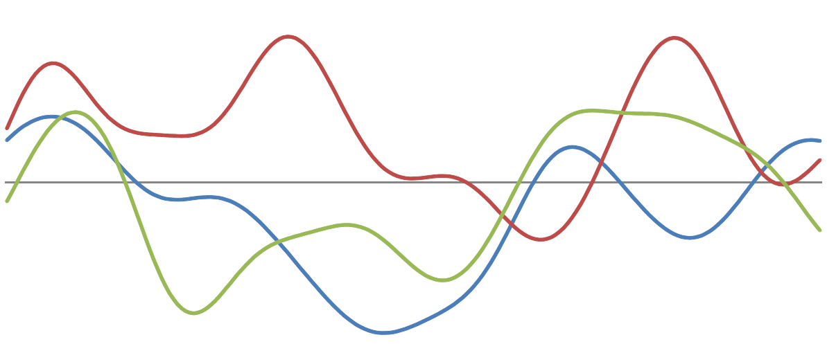
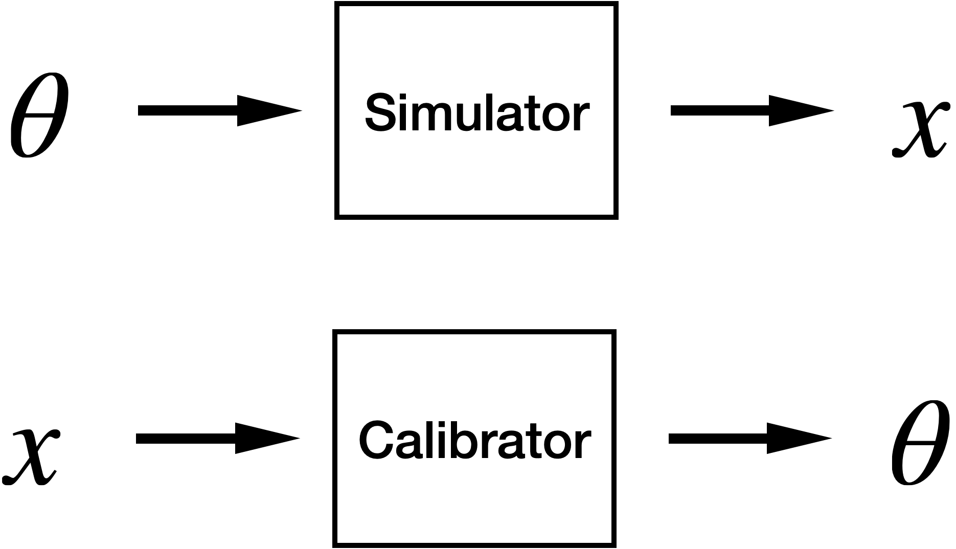
Typically hard because
- No access to the likelihood.
- Simulator is slow to run.
- Large parameter space.
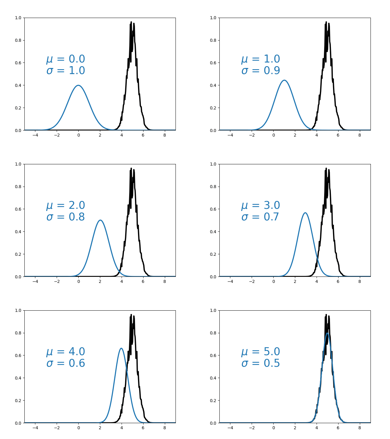
Variational Inference
- Assume posterior can be approximated by a parameterised distribution.
- Optimise for best parameters using gradient
(Generalized) Variational Inference
Knoblauch et al (2019)

ABM
Prior
(Generalized) posterior
(Generalized) Variational Inference
Optimization problem
Assume posterior approximated by variational family
Distance between ABM output and data
Divergence posterior - prior
How to optimize q?
Choose parametric family of distributions (e.g., Normal)
How to optimize q?
Need to compute the gradient
Score function estimator
Monte Carlo
gradient estimation
Mohamed et al (2020)
Path-wise estimator
Reparameterization
Score function estimator
Path-wise estimator
- Unbiased
- Typically high variance
- Does not require differentiable simulator
- Unbiased*
- Low(er) variance
- Requires differentiable simulator
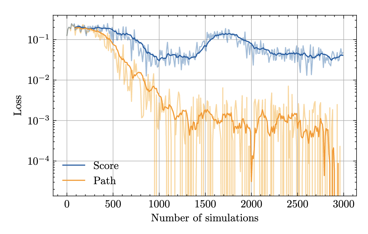
"Gradient assisted calibration of financial agent-based models" Dyer et al. (2023)
How to build differentiable
Agent-Based Models
Differentiable simulators
Numerical differentiation
Inaccurate
Automatic differentiation

def f(x1)
	t1 = x1 * x1
    t2 = t1 * t1
return t2 * t22
4
16
256
Idea:
Decompose program into basic operations that we can differentiate
Automatic differentiation
Reverse mode AD

2
4
16
256
Forward mode AD

2
4
16
256
Automatic differentiation
Reverse mode AD

2
4
16
256
Forward mode AD

2
4
16
256
Forward vs Reverse
Multiple outputs
def f(x1)
	t1 = x1 * x1
    t2 = t1 * t1
    return [t2, t2, t2]
Reverse needs 3 full model evaluations!
Forward can amortize
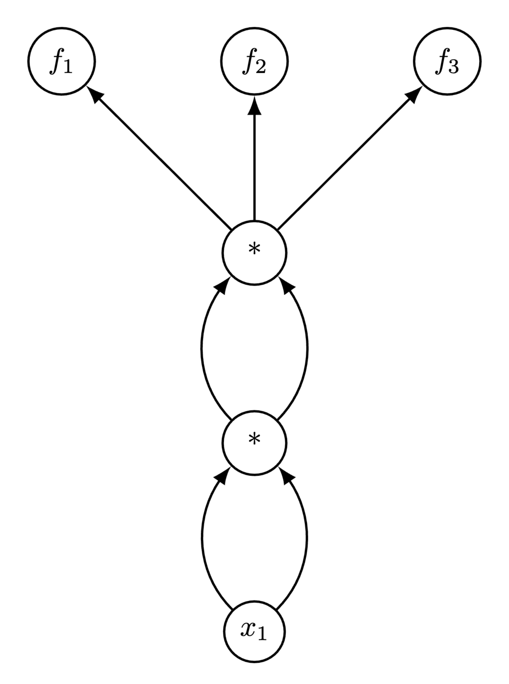
Forward vs Reverse
Multiple inputs
def f(x1, x2, x3)
	t1 = x1 * x2 * x3
    t2 = t1 * t1
    return t2 * t2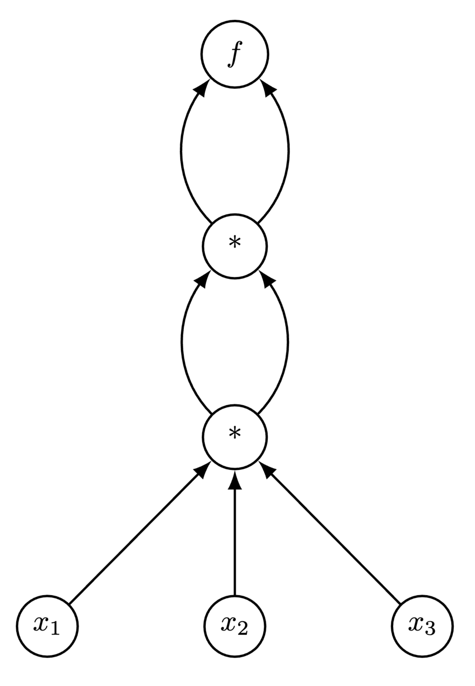
Forward needs 3 full model evaluations!
Reverse can amortize
Forward vs Reverse
Reverse mode preferred for deep learning
However
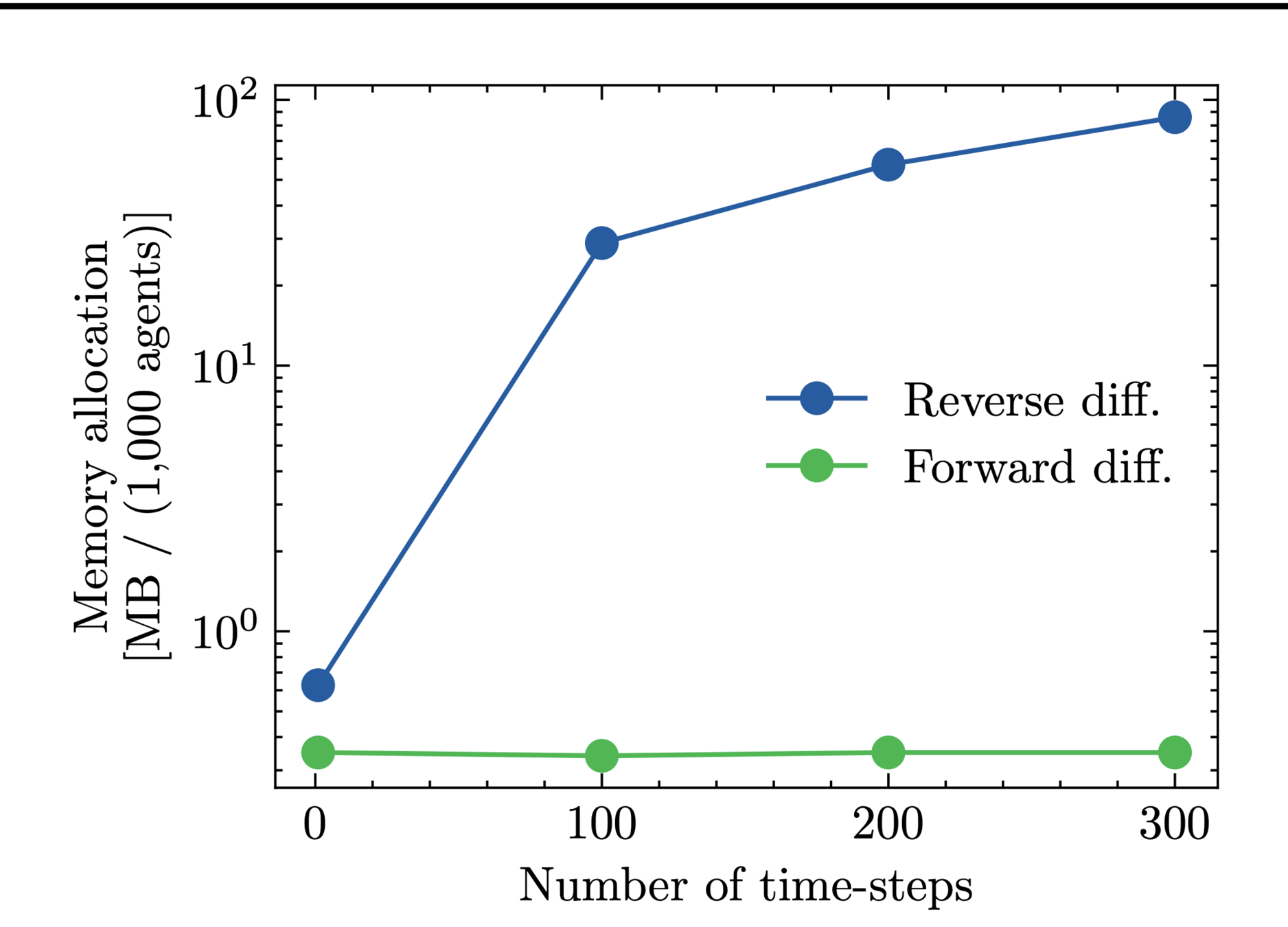
Quera-Bofarull et al. "Some challenges of calibrating differentiable agent-based models"
Reverse mode needs to store computational graph!
Can blow up in memory
Differentiating through randomness
What about discrete distributions?
Option 1: Straight-Through
Just assign a gradient of 1.
Works if program is linear
Bengio et al. (2013)
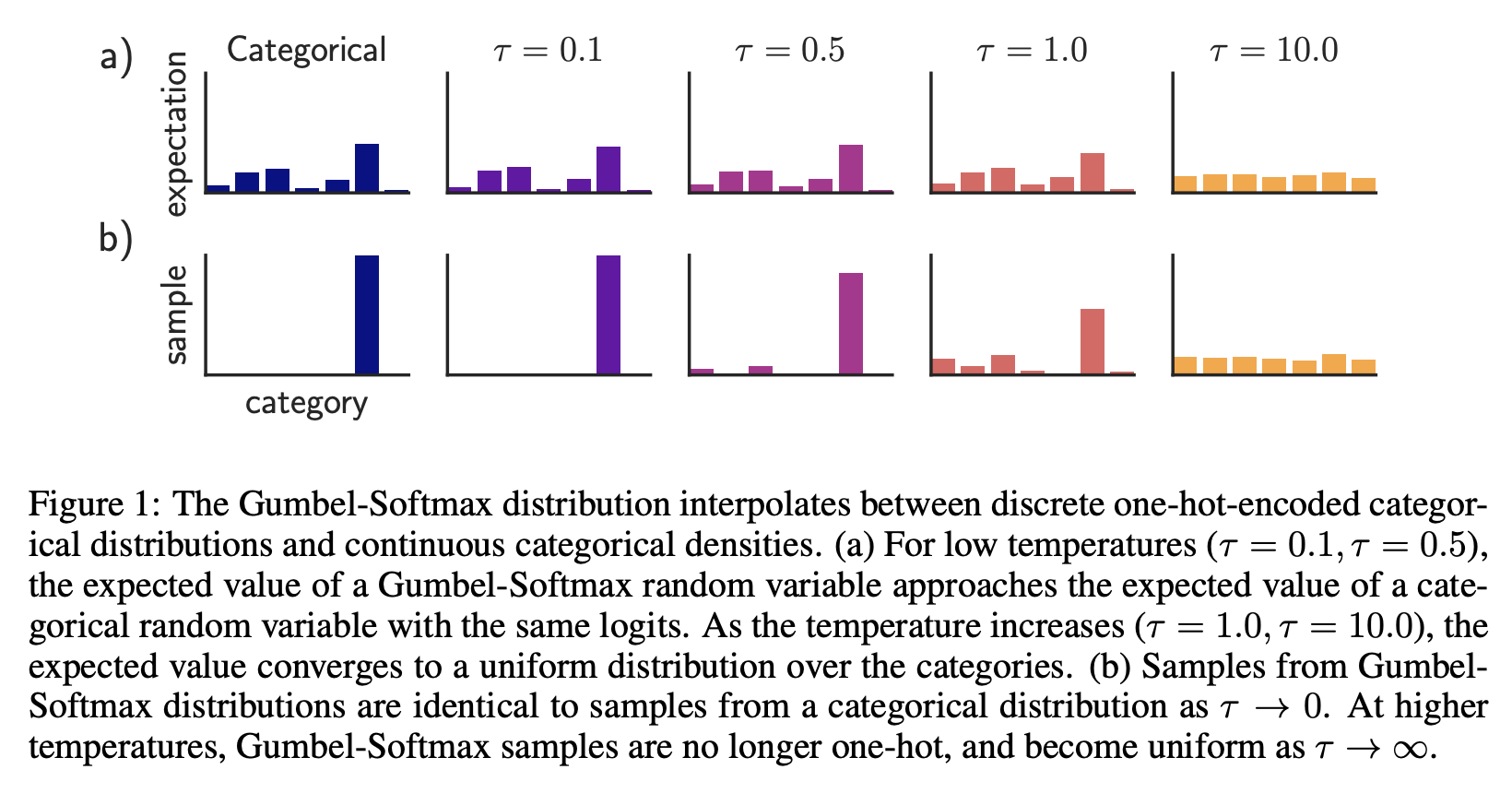
Option 2: Gumbel-Softmax
Jang et al. (2016)
Bias vs Variance tradeoff
Option 3: Smooth Perturbation analysis
StochaticAD.jl -- Arya et al. (2022)

Unbiased!
So does it work?

arnau.ai/blackbirds
Multiple examples of differentiable ABMs in PyTorch and Julia
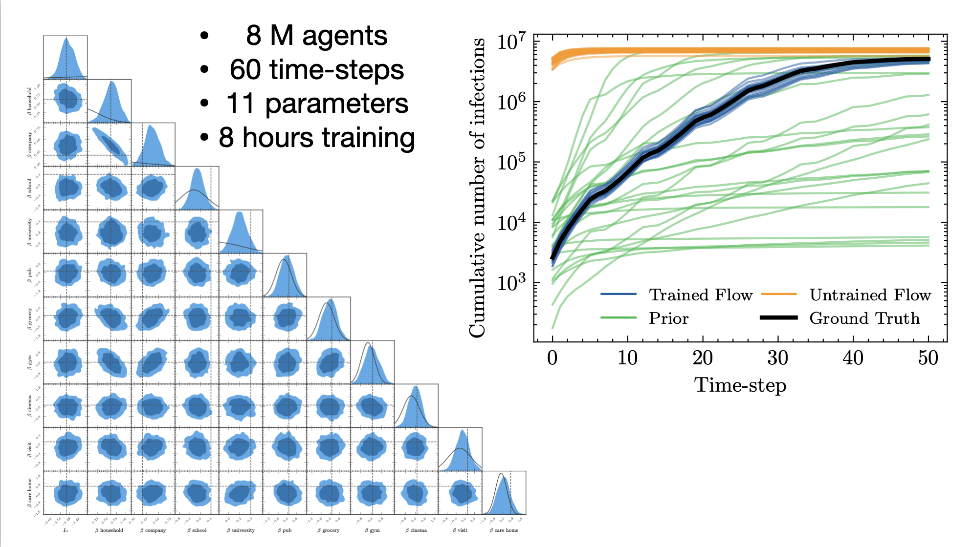
JUNE epidemiological model
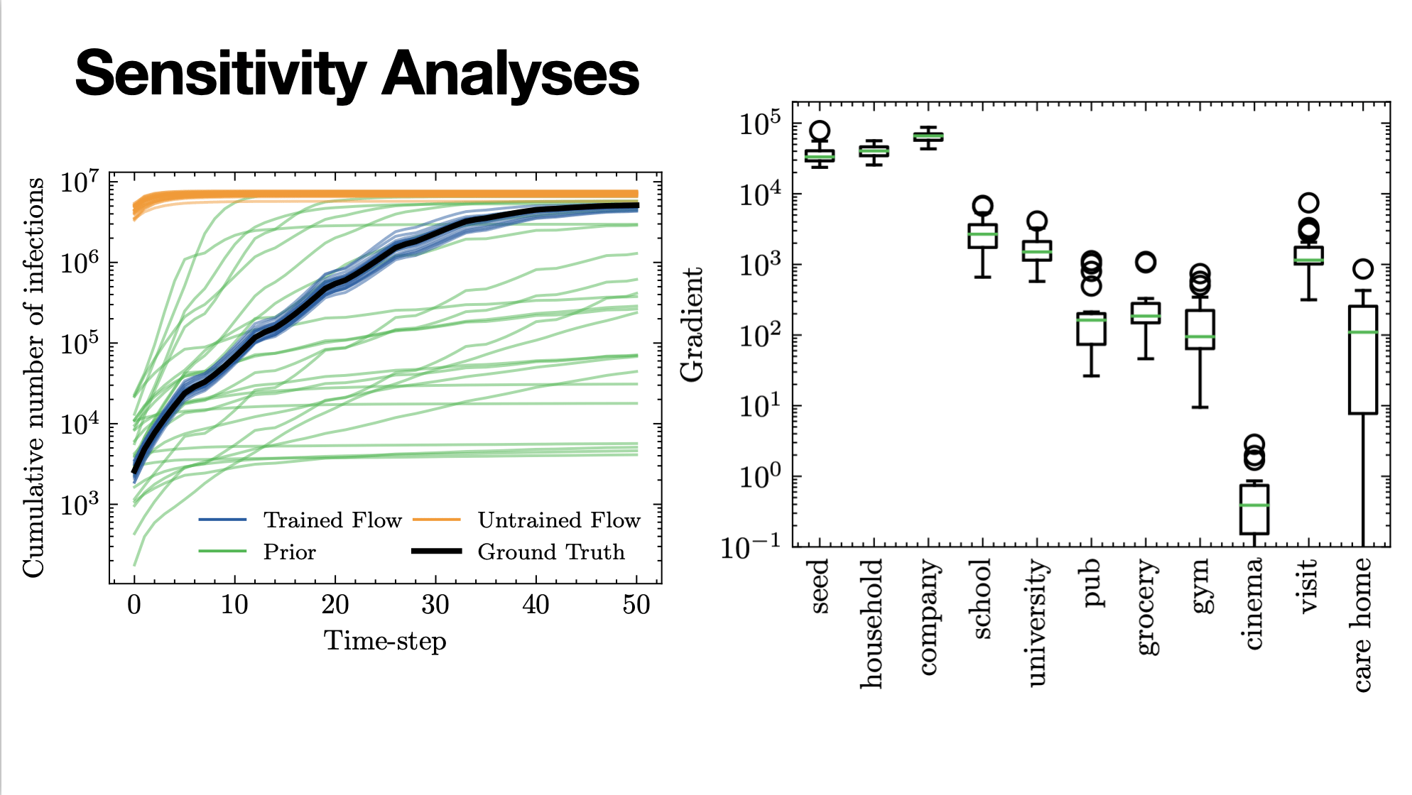
Reverse-mode gives us senstivity analysis for free
Summary
-
Generalized Variational Inference promising route to calibrate differentiable ABMs.
-
Differentiable ABMs can be built using Automatic Differentiation
-
Automatic Differentiation provides O(1) sensitivity analysis.
Slides and papers:
www.arnau.ai/talks
Diff ABM examples:
www.arnau.ai/blackbirds
Backup slides
Symbolic differentiation
function f(x1)
	t1 = x1 * x1
    t2 = t1 * t1
    return t2 * t2
end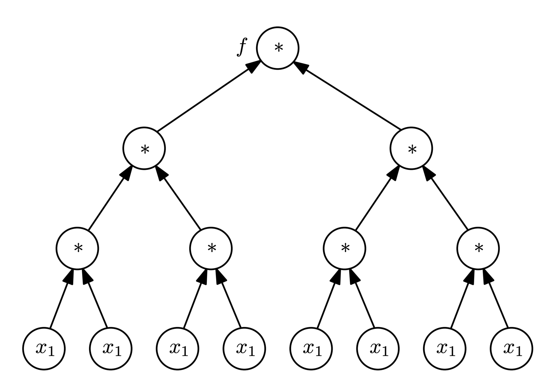
Symbolic differentiation

Hard-code calculus 101 derivatives
Recurrently go down the tree via chain rule
Inefficient representation
Exact result
Automatic differentiation


DifferentiableAgent-Based Models
By arnauqb
DifferentiableAgent-Based Models
- 536


