Health Data Science Meetup
November 18, 2016

Introduction
Multilayer Perceptrons
Implementations in Python
The Limits of Traditional Computer Programs
Image from MNIST handwritten digit dataset
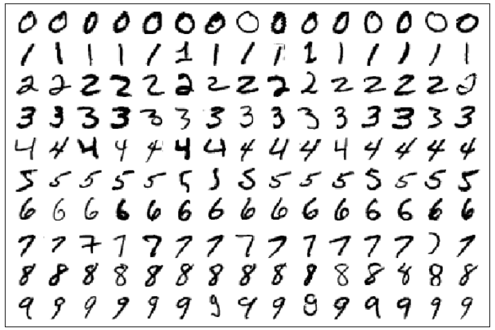
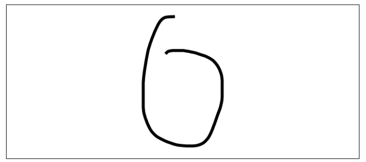
A zero that is difficult to distinguish from a six algorithmically
- How to distinguish between threes and fives?
- Or between fours and nines?
We don't know what program to write because we don't know how it's done by our brains
Machine Learning
- Many things we learn in school have a lot in common with traditional computer programs:
how to multiply numbers, solve equations, take derivatives
- The things we learn at an extremely early age, the things we find most natural, are learned by example, not by formula:
recognize a dog
- In other words, when we were born, our brains provided us with a model that described how we would be able to see the world
- as we grew up, that model would take in our sensory inputs and make a guess about what we're experiencing
- if that guess is confirmed by our parents, our model would be reinforced
- over our lifetime, our model becomes more and more accurate as we assimilate billions of examples
Machine Learning
- Machine learning is predicated on this idea of learning from example
- Instead of teaching a computer a massive list rules to solve the problem, we give it a model with which it can evaluate examples and a small set of instructions to modify the model when it makes a mistake

Let's define our model to be a function
h(x,\theta)
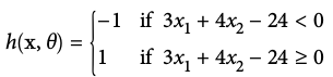
Another Example
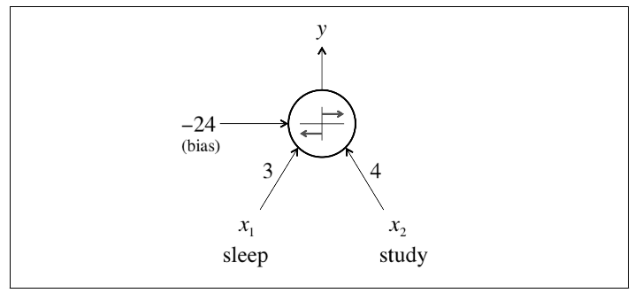
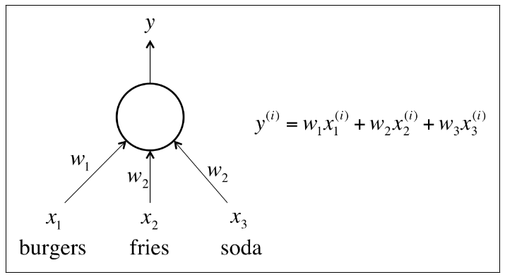
- To predict exam performance (above or below average) based on the number of hours of sleep we get and the number of hours we study in the previous day
- We collect a lot of data
- Our goal might be to learn a model with parameter vector
such that:
h(x,\theta)
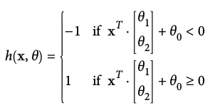
A linear perceptron
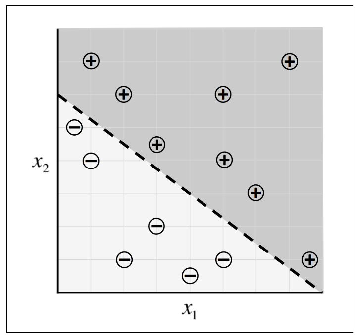
Deep Learning
- As we move on to much complex problems, our data
- not only becomes extremely high dimensional
- the relationships we want to capture also become highly nonlinear
- To accommodate this complexity, recent research in machine learning has attempted to build models that highly resemble the structures utilized by our brains
- Commonly referred to as deep learning, which has had spectacular success in tackling problems in computer vision and natural language processing
- not only far surpass other kinds of machine learning algorithm
- also rival the accuracies achieved by humans
Multilayer Perceptrons
Introduction
-
Neural Networks
- A field of study that investigates how simple models of biological brains can be used to solve difficult computational tasks (i.e. predictive modeling in machine learning)
- the goal is not to create realistic model of the brain
- develop robust algorithms and data structures that can be used to model difficult problems
- NNs are capable of learning any mapping function and have been proven to be a universal approximation algorithm
- the predictive capability of NNs comes from the hierarchical/multilayered structure of the networks
- the data structure can pick out features at different scales or resolutions and combine them into higher-order features
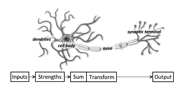
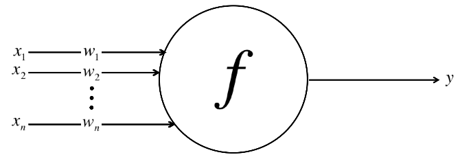
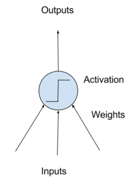
Perceptron
- Perceptron:
- a single neuron model that was a precursor to larger neural networks
- neuron
- neuron weights
- activation
- Neuron: the building block for NNs
- simple computational units that have weighted input signals and produce an output signal using an activation function
Perceptron
- Neuron weights:
- similar to the coefficients used in a regression equation
- like linear regression, each neuron also has a bias which can be thought of as an input that always has the value 1.0 and it too must be weighted (e.g. a neuron may have 2 inputs, and it requires 3 weights)
- weights are often initialized to small random values (i.e. 0~0.3)
- Activation:
- the weighted inputs are summed and passed through an activation function (also called a transfer function)
- it governs the threshold at which the neuron is activated and the strength of the output signal
- historically, simple step activation functions were used (e.g. if the summed input was above a threshold, say 0, then the neuron would output a value of 1, otherwise, output a -1)
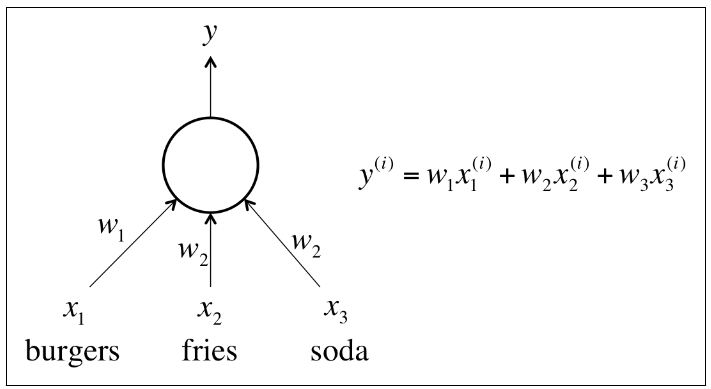
Expressing Linear Perceptrons
Feed-forward Neural Networks
- Single neurons are not expressive enough to solve complicated learning problems
- The neurons in the human brain are organized in layers
- information flows from one layer to another
- sensory input is converted into conceptual understanding

Feed-forward NNs:
- connections only traverse from a lower layer to a higher layer
- no connections between neurons in the same layer
- no connections that transmit data from a higher layer to a lower layer
Linear Activation

- Linear activation is easy to compute with, but has serious limitations
- Any feed-forward NN consisting of only linear activation can be expressed as a NN with no hidden layers
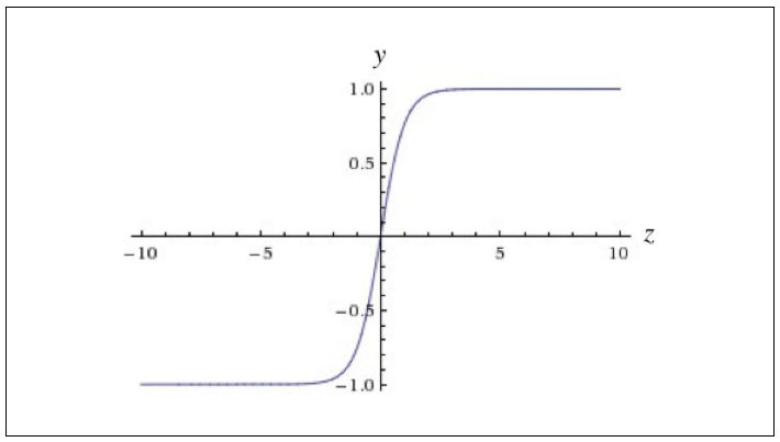
Nonlinear Activation
- In order to learn complex relationships, we need to use activation functions that employ some sort of nonlinearity
Logistic function / Sigmoid function: 0~1
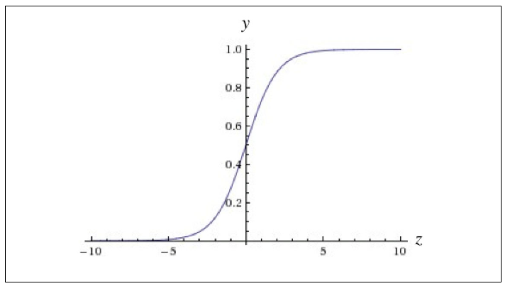
f(z)=1/(1+e^{-z})
f(z)=Tanh(z)
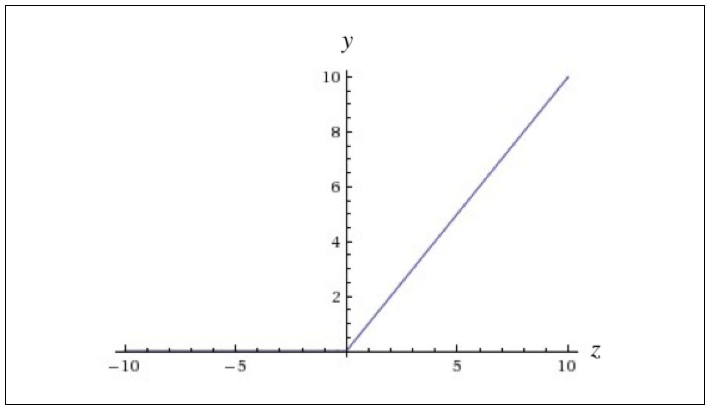
f(z)=max(0,z)
Hyperbolic tangent (Tanh) function: -1~1
ReLU (rectified linear unit) function
Networks of Neurons
- Neurons are arranged into networks of neurons:
- a row of neurons is called a layer
- the architecture of the neurons in the network is often called the network topology
- Input or Visible Layer:
- the bottom layer, which takes input from the dataset
- usually with one neuron per feature in the dataset
- Hidden Layers:
- not directly exposed to the input
- the simplest network structure is to have a single neuron in the hidden layer that directly outputs the value
- deep learning can refer to having many hidden layers in NN
- Output Layer:
- the final hidden layer
- the choice of activation function in the output layer is constrained by the type of problem that you are modeling
- e.g. single output neuron with no activation function for regression problem, single output neuron with a sigmoid function for binary classification problem, softmax output layer for multiclass classification problem

Training Feed-Forward Neural Networks
- How do we figure out the weights for all the connections in our NN?
- Training:
- show the NN a large number of training examples
- iteratively modify the weights to minimize the errors we make on the training examples
- after enough examples, we expect that our NN will be quite effective at solving the task it's been trained to do
Single Perceptron
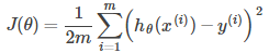
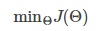
Cost Function:

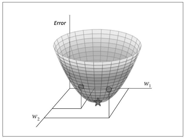
Gradient Descent:
- Taking the derivative of our cost function
- The slope of the tangent is the derivative at that point and it will give us a direction to move towards
- We make steps down the cost function in the direction with the steepest descent, and the size of each step is determined by the parameter α, which is called the learning rate
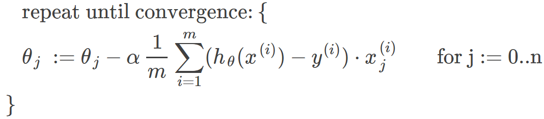
Gradient Descent
The gradient descent algorithm is:
repeat until convergence:
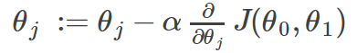
Learning Rate
- Picking the learning rate is a hard problem:
- if too small, we risk taking too long during the training process
- if too big, we are likely start diverging away from the minimum
There are various optimization techniques that utilize adaptive learning rates to automate the process of selecting learning rates
Multilayer Perceptrons
L
s_l
K
total number of layers in the network
number of units (exclude the bias unit) in layer l
number of output units/classes
h_\theta(x)_k
the output
k^{th}


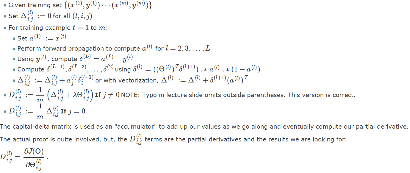
Backpropagation Algorithm
- "Backpropagation" is NN terminology for minimizing our cost function
- Our goal is to compute:
- we want to minimize our cost function using an optimal set of parameters in theta
- Need to compute:
-
-

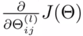
Gradient computation
- Given one training example (x,y)
- Forward propagation:
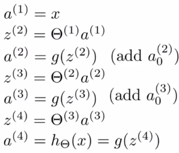
a^{(1)}
a^{(2)}
a^{(3)}
a^{(4)}
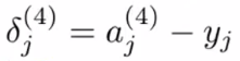
Gradient computation: Backpropagation algorithm
- Intuition: "error" of node j in layer l
- For each output unit (e.g. layer L=4):
- No

a^{(1)}
a^{(2)}
a^{(3)}
a^{(4)}
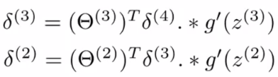
=a^{(3)}.*(1-a^{(3)})
\delta^{(1)}
\delta^{(4)}
\delta^{(2)}
\delta^{(3)}
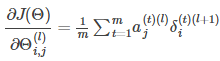
Backpropagation algorithm
Training Networks
- Data Preparation:
- data must be numerical (one-hot encoding for categorical features)
- NNs require the input to be scaled in a consistent way (e.g. normalization)
-
Stochastic Gradient Descent:
- classical training algorithm for NNs
- one row of data is exposed to the network at a time as input
- the network processes the input upward activating neurons as it goes to finally produce an output value (forward propagation)
- the output of the network is compared with the expected output and an error is calculated
- this error is then propagated back through the network, one layer at a time, and the weights are updated according to the amount that they contributed to the error (back propagation algorithm)
- the process is repeated for all of the examples in training data
- one round of updating the network for the entire training dataset is called an epoch
Batch Gradient Descent
- Batch Gradient Descent:
- we use our entire dataset to compute the error surface and then follow the gradient to take the path of steepest descent
- for simple quadratic error surface, this works quite well
- but in most cases, the error surface is a lot more complicated

Stochastic Gradient Descent
(Online Learning)
- Stochastic Gradient Descent:
- at each iteration, the error surface is estimated only with respect to a single example
- dynamic error surface
- descending on this stochastic surface significantly improves our ability to avoid local minima
Major limitation:
- looking at the error incurred one example at a time may not be a good enough approximation of the error surface
- make it take a significant amount of time
Mini-batch Gradient Descent
(Batch Learning)
- At each iteration, the error surface is estimated using some subset of the total dataset (instead of just a single example)
- It strike a balance between the efficiency of batch gradient descent and the local-minima avoidance afforded by stochastic gradient descent
- The subset is called a mini-batch
- The size of the mini-batch is another hyperparameter in addition to learning rate
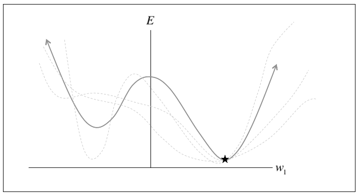
Beyond Gradient Descent
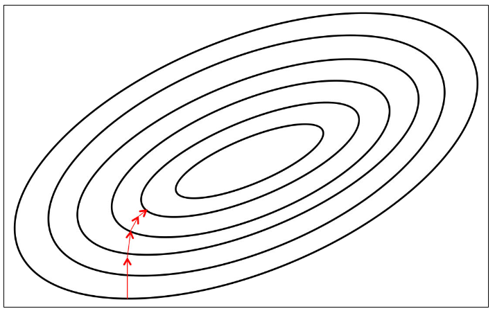
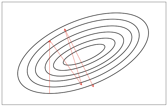
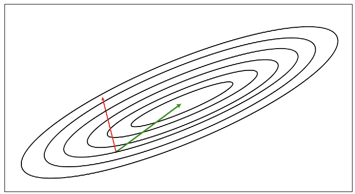
- The most critical challenge: finding the correct trajectory to move in
- The gradient is not usually a very good indicator of the good trajectory
- only when the contours are perfectly circular does the gradient always point in the direction of the local minimum
- if the contours are extremely elliptical (most deep networks), the gradient can be as in accurate as 90 degrees
- As we move along the direction of steepest descent, the direction of the gradient changes
- we can quantify how the gradient changes under our feet as we move in a certain direction by computing the second derivatives
- however, it turns out difficult to compute
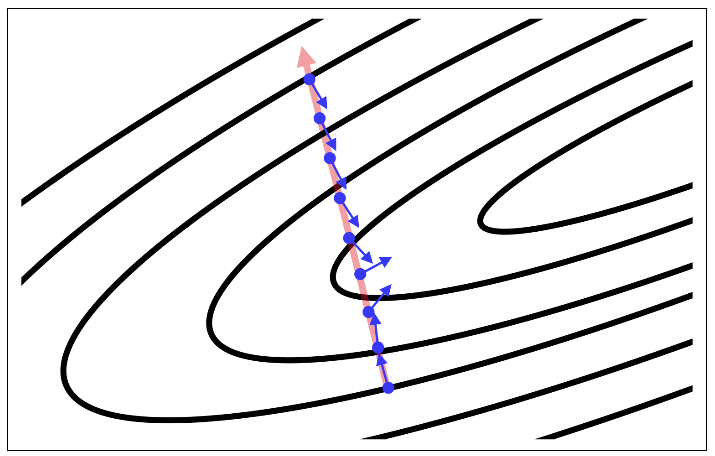
Momentum-Based Optimization
- If we think about how a ball rolls down a hilly surface:
- driven by gravity, the ball eventually settles into a minima on the surface
- for some reason, it does not suffer from the wild fluctuations and divergences that happen during gradient descent
- why?
- Unlike in gradient descent (which only uses the gradient), there are two major components that determine how a ball rolls down an error surface:
- acceleration (gradient)
- velocity
- Velocity serves as a form of memory
- it allows us to more effectively accumulate movement in the direction of the minimum while canceling out oscillating accelerations in orthogonal directions
- The momentum-based optimization is an analog for velocity
- we use the momentum hyperparameter m to determine what fraction of the previous velocity to retain in the new update and add this "memory" of past gradients to our current gradient
Learning Rate Adaptation
- Selecting the learning rate is another major challenge for training deep NN
- Learning rate adaption:
- the optimal learning rate is appropriately modified over the span of learning to achieve good convergence properties
- Three most population adaptive learning rate algorithms:
- AdaGrad: adapt global learning rate over time using an accumulation of the historical gradients
- RMSProp: exponentially weighted moving average of gradients
- Adam: combining momentum and RMSProp
Preventing Overfitting
- L1 and L2 regularization
- Max norm constraints
- similar goal as L1 and L2 regularization to restrict theta from becoming too large
- enforce an absolute upper bound on the magnitude of the incoming weight vector for every neuron and use projected gradient descent to enforce the constraint
- anytime a gradient descent step moved the incoming weight vector such that
we project the vector back onto the ball with radius c (e.g. 3 and 4 are typical c)
- the updates to the weights are always bounded so that the parameter vector cannot grow out of control, even when the learning rates are too high
- Dropout:
- proposed by Srivastava et al. in 2014
- randomly selected neurons are ignored during training
- their contribution to the activation of downstream neurons is temporally removed on the forward pass and any weight updates are not applied to the neuron on the backward pass
- the network becomes less sensitive to the specific weights of neurons, which in turn results in a network that is capable of better generalization and is less likely to overfit the training data
||w||_2>c
Hyperparameter Tuning and Optimizer Selection
- Most popular algorithms currently:
- minibatch gradient descent
- minibatch gradient with momentum
- RMSProp
- RMSProp with momentum
- Adam
- The best way to push the model performance for deep learning:
- not by building more advanced optimizers to wrangle with nasty error surfaces
- instead, most breakthroughs in deep learning have been obtained by discovering architectures that are easier to train: e.g. convolutional NNs, recurrent NNs
Prediction
- Once a NN has been trained, it can be used to make predictions
- The network topology and the final set of weights is all that you need to save from the model
- Predictions are made by providing the input features to the network and performing a forward-pass allowing it to generate an output that you can use as a prediction
Implementations
Deep Learning Package Zoo

Python, R, Julia, and Scala
Lua
Python


Python

Java

Python
Keras

- A minimalist Python library for deep learning that can run on top of Theano or TensorFlow
- Developed to make developing deep learning models as fast and easy as possible
Select the correct binaries to install
# Ubuntu/Linux 64-bit, CPU only, Python 2.7
$ export TF_BINARY_URL=https://storage.googleapis.com/tensorflow/linux/cpu/tensorflow-0.11.0-cp27-none-linux_x86_64.whl

# Ubuntu/Linux 64-bit, GPU enabled, Python 2.7
# Requires CUDA toolkit 8.0 and CuDNN v5. For other versions, see "Install from sources" below.
$ export TF_BINARY_URL=https://storage.googleapis.com/tensorflow/linux/gpu/tensorflow-0.11.0-cp27-none-linux_x86_64.whl

# Mac OS X, CPU only, Python 2.7:
$ export TF_BINARY_URL=https://storage.googleapis.com/tensorflow/mac/cpu/tensorflow-0.11.0-py2-none-any.whl

# Mac OS X, GPU enabled, Python 2.7:
$ export TF_BINARY_URL=https://storage.googleapis.com/tensorflow/mac/gpu/tensorflow-0.11.0-py2-none-any.whl
Install TensorFlow
# Python 2
$ pip install --upgrade $TF_BINARY_URL
TensorFlow (Linux/OS X)
$ pip install keras
Develop Models on GPUs In the Cloud
-
UF Research Computing (HiperGator/ResVault)
-
Amazon Web Service (AWS)
- Setup AWS account
- Launch server instance
- Login and run codes
- Close server instance
- Free options:
- AWS EC2 750 hours per month of t2.micro instance usage (Expires 12 months after sign-up)
- GitHub Education Student Developer Pack ($150 AWS credits)
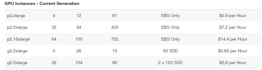
$150 credits = ~230 hours usage of g2.2xlarge
Launch Server Instance
- Login to AWS console
- Click on EC2
- Select N. California from the drop-down in the top right hand corner
- Click Launch Instance button
- Click Community AMIs
- Enter ami-125b2c72 in the Search Community AMIs search box
- Click Select button
- Select g2.2xlarge hardware
- Click Review and Launch
- Click the Launch button
- Select Key Pair
- Open a Terminal and change directory to where the key pair is stored
- Restrict the access permissions on your key pair file:
chmod 600 nameofkeypair.pem - Click Launch Instances
- Click View Instances to review the status of your instance
Login, Configure and Run
- Copy the Public IP
- Open a Terminal and change directory to where your key pair is stored. Login to your server using SSH:
ssh -i nameofkeypair.pem ubuntu@52.53.186.1 - If prompted, type yes and press enter
- Update Keras:
pip install --upgrade --no-deps keras==1.1.1 - Configure Theano:
vi ~/.theanorc - Copy and paste the following configuration and save the file:
[global]
device = gpu
floatX = float32
optimizer_including = cudnn
allow_gc = False
[lib]
cnmem=.95 - Confirm Theano is working:
python -c "import theano; print(theano.sandbox.cuda.dnn.dnn_available())" - You should see:
Using gpu device 0: GRID K520 (CNMeM is enabled)
True - Enable Jupyter Notebook (optional, only if you want to use the jupyter notebook)
Close Your EC2 Instance
- Log out of your instance at the terminal:
exit - Log in to your AWS account with your web browser
- Click EC2
- Click Instances from the left-hand side menu
- Select your running instance from the list
- Click Actions button and select Instance State and choose Terminate
Next Meetup: CNN and RNN
Dec 5, 2016
9-11 AM
HDS Meetup 11/18/2016
By Hui Hu
HDS Meetup 11/18/2016
Slides for the Health Data Science Meetup


