k-means, LASSO, and Random Forest
Applications for Machine Learning Working Group from
The Mortality and Medical Costs of Air Pollution: Evidence from Changes in Wind Direction
paper Summary
- Measure the impact of fine particulate matter pollution (PM 2.5) on mortality and healthcare use
- IV approach that leverages local wind changes on (non-local) pollution
- Use machine learning to simulate life-years lost (LYL) due to pollution exposure
- K-means for data cleaning
- Hazard rate refinement using high-dimensional datasets
- LASSO
- Random Forest
- Chernozhukov et al. (2018) ML for heterogeneity (I won't cover, highly technical that would probably need its own session)
Empirical strategy
- How to estimate how long someone has to live?
- Cox proportional hazards model
Empirical strategy
- How to estimate how long someone has to live?
- Cox proportional hazards model:
h(t_i|x_i,\beta)=\underbrace{h_0(t_i)}\underbrace{exp[x_i'\beta]}
Baseline survival rate
Individual characteristics
Empirical strategy
- How to estimate how long someone has to live?
- Cox proportional hazards model:
h(t_i|x_i,\beta)=\underbrace{h_0(t_i)}\underbrace{exp[x_i'\beta]}
Baseline survival rate
Individual characteristics
>1: increased risk
<1: decreased risk
Empirical strategy
- How to estimate how long someone has to live?
- Cox proportional hazards model:
h(t_i|x_i,\beta)=\underbrace{h_0(t_i)}\underbrace{exp[x_i'\beta]}
Baseline survival rate
Individual characteristics
Estimate with log partial likelihood
Empirical strategy
- How to estimate how long someone has to live?
- Cox proportional hazards model:
h(t_i|x_i,\beta)=\underbrace{h_0(t_i)}\underbrace{exp[x_i'\beta]}
Estimate with log partial likelihood
\ln L(\beta) = \sum^N_{i=1} \delta_i \left[ x_i'\beta - \ln \sum_{j \in R(t_i)} \exp[x_j'\beta] \right]
Empirical strategy
- How to estimate how long someone has to live?
- Cox proportional hazards model:
h(t_i|x_i,\beta)=\underbrace{h_0(t_i)}\underbrace{exp[x_i'\beta]}
\ln L(\beta) = \sum^N_{i=1} \delta_i \left[ x_i'\beta - \ln \sum_{j \in R(t_i)} \exp[x_j'\beta] \right]
Observe death =1
The risk set: the entire set of subjects at risk at time i
Characteristics of those individuals
Empirical strategy
- How to estimate how long someone has to live?
- Cox proportional hazards model:
h(t_i|x_i,\beta)=\underbrace{h_0(t_i)}\underbrace{exp[x_i'\beta]}
\ln L(\beta) = \sum^N_{i=1} \delta_i \left[ x_i'\beta - \ln \sum_{j \in R(t_i)} \exp[x_j'\beta] \right]
Maximize this, or rather, minimize the negative of this
Intuitively, choose β such that it weights riskier characteristics more
Sources: https://en.wikipedia.org/wiki/Proportional_hazards_model and http://www.sthda.com/english/wiki/cox-proportional-hazards-model
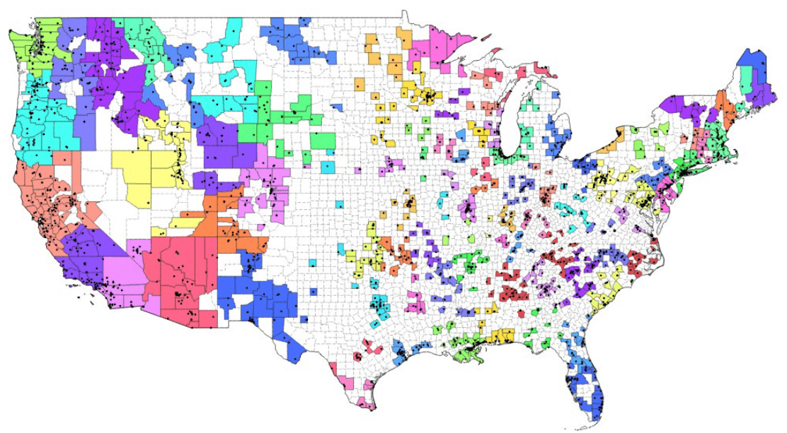
Problem:
- There are nearly 1,400 PM 2.5 monitors in the country, but they are sparsely placed.
- Locally produced pollution will generate data noise based on proximity to certain monitors.
- Local pollution unlikely to reach all individuals in a given area.
Measurement Error!
Problem:
- There are nearly 1,400 PM 2.5 monitors in the country, but they are sparsely placed.
- Locally produced pollution will generate data noise based on proximity to certain monitors.
- Local pollution unlikely to reach all individuals in a given area.
Measurement Error!
Focus on systematic pollution by grouping together monitors in multiple counties
Problem:
- There are nearly 1,400 PM 2.5 monitors in the country, but they are sparsely placed.
- Locally produced pollution will generate data noise based on proximity to certain monitors.
- Local pollution unlikely to reach all individuals in a given area.
- Unsupervised machine learning technique
- Partitions data around associated centroids, based on the number of clusters k chosen in advance
- Simple method (the "OLS of clustering") of classifying geospatial or even data that might not have interpretable distance (e.g. Spotify songs)
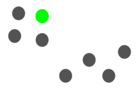
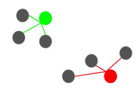
k-means clustering
If we want to be more sophisticated than just picking the monitor groups ourselves...
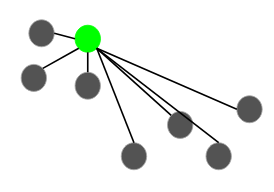
The algorithm
- (Possibly, especially if not geospatial)
scale and normalize features - Select K points for initial centroids
-
Begin while loop
- Form K clusters by assigning all
points to the closest centroid - Recompute the centroid for each
cluster
- Form K clusters by assigning all
- Stop loop when centroids are stable (usually fairly rapidly but complexity increases in data points, clusters K, and features)
Source: https://github.com/jgscott/ECO395M
The algorithm
- (Possibly, especially if not geospatial)
scale and normalize features - Select K points for initial centroids
-
Begin while loop
- Form K clusters by assigning all
points to the closest centroid - Recompute the centroid for each
cluster
- Form K clusters by assigning all
- Stop loop when centroids are stable (usually fairly rapidly but complexity increases in data points, clusters K, and features)
- Might need to spot-check clusters, if possible
- Each iteration will be different
- Set seed, or
- Use 20+ starts (many packages will choose the start with the lowest within-cluster variation), or
- Use a different initialization strategy K-means++
Some Issues
Choose initial
centroid
K-means++
Choose initial
centroid
Compute distance to x's
K-means++
Choose initial
centroid
Compute distance to x's
Probabilistically weight furthest as next centroid
K-means++
Choose initial
centroid
Compute distance to x's
Probabilistically weight furthest as next centroid
Stop when you reach K centroids
K-means++
Source: https://www.analyticsvidhya.com/blog/2019/08/comprehensive-guide-k-means-clustering/
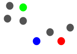
Toy Example

Problem:
- How do we know what is important for how long someone will live?
- We could use some economic intuition to guess, but this is subjective
Problem:
- How do we know what is important for how long someone will live?
- We could use some economic intuition to guess, but this is subjective
- Huge dataset with more than 1000 variables, so simply testing one against another is infeasible
Problem:
- How do we know what is important for how long someone will live?
- We could use some economic intuition to guess, but this is subjective
- Huge dataset with more than 1000 variables, so simply testing one against another is infeasible
Reduce Dimensions
Problem:
- How do we know what is important for how long someone will live?
- We could use some economic intuition to guess, but this is subjective
- Huge dataset with more than 1000 variables, so simply testing one against another is infeasible
Reduce Dimensions
Machine Learning can train on data to select important variables
Problem:
- How do we know what is important for how long someone will live?
- We could use some economic intuition to guess, but this is subjective
- Huge dataset with more than 1000 variables, so simply testing one against another is infeasible
- Least absolute shrinkage and selection operator
- Makes explicit the tradeoff between choosing covariates to minimize the differences between predicted y and observed y (goodness of fit) and selecting on too many variables (overfitting)
- Can be applied easily to linear regression, proportional hazard, and many other empirical strategies, when it is not clear what is important
LASSO
Solution 1:
LAsso
- LASSO takes the generic form
where dev is closeness of fit and pen is a penalty function on any beta that is non-zero.
- In linear regression using L1 regularization as the penalty, we get a Lagrangian optimization problem that takes the form
\min_{\beta \in \R^p} \frac{1}{n} \text{dev} +\lambda \text{pen}(\beta)
\min_{\beta \in \R^p} \left( \frac{1}{n} (y-X\beta)^2 +\lambda \sum_\beta|\beta| \right)
\min_{\beta \in \R^p} \frac{1}{n} \text{dev} +\lambda \text{pen}(\beta)
\min_{\beta \in \R^p} \left( \frac{1}{n} (y-X\beta)^2 +\lambda \sum_\beta|\beta| \right)
How is this Machine Learning?
\min_{\beta \in \R^p} \frac{1}{n} \text{dev} +\lambda \text{pen}(\beta)
\min_{\beta \in \R^p} \left( \frac{1}{n} (y-X\beta)^2 +\lambda \sum_\beta|\beta| \right)
How is this Machine Learning?
- Chosen value of lambda is data-dependent
- Apply validation tools (e.g. cross-validation to determine optimal value)
\min_{\beta \in \R^p} \left( \frac{1}{n} (y-X\beta)^2 +\lambda \sum_\beta|\beta| \right)
How is this Machine Learning?
- Chosen value of lambda is data-dependent
- Apply validation tools (e.g. cross-validation to determine optimal value)
algorithm
- Start with \( \lambda_1 \) so big that any \( \hat{\beta} =0 \)
- For each iteration update \( \hat{\beta} \) to be optimal under \( \lambda_t < \lambda_{t-1} \)
- Use a testing set to pick the best \( \lambda \)
- Need a rule, such as minimum \( \lambda \) or 1se rule (pick the largest \( \lambda \) still within 1 standard error of minimum)
Source: https://github.com/jgscott/ECO395M
Toy Example

Results
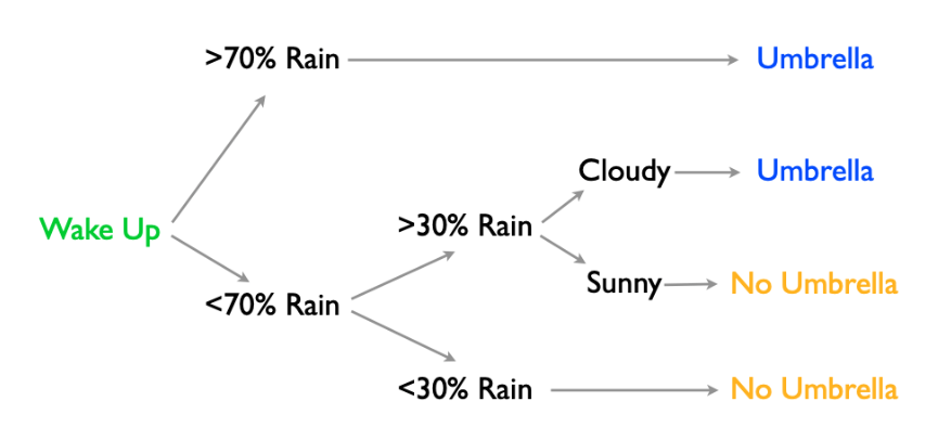
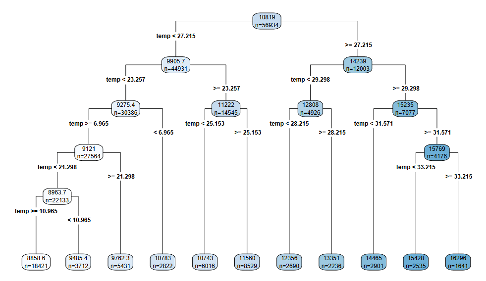
- Trees are sequential decision nodes that branch on inputs to predict the output
Random forest
Solution 2:
Source: https://github.com/jgscott/ECO395M
- Trees are sequential decision nodes that branch on inputs to predict the output
Random forest
Source: https://github.com/jgscott/ECO395M
- Trees are sequential decision nodes that branch on inputs to predict the output
- Based on previous data, use to either
- Categorize: \( P(Y|X) \)
- Estimate: \( E(Y|X) \)
- For numeric x, the decision rule is x<c
Random forest
Source: https://github.com/jgscott/ECO395M
- Trees are sequential decision nodes that branch on inputs to predict the output
- Based on previous data, use to either
- Categorize: \( P(Y|X) \)
- Estimate: \( E(Y|X) \)
- For numeric x, the decision rule is x<c
Random forest
Source: https://github.com/jgscott/ECO395M
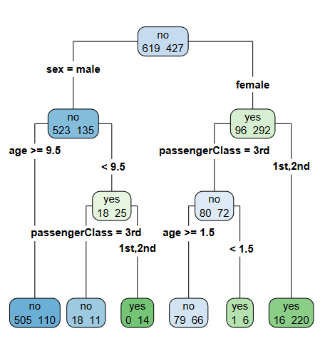
- Trees are sequential decision nodes that branch on inputs to predict the output
- Based on previous data, use to either
- Categorize: \( P(Y|X) \)
- Estimate: \( E(Y|X) \)
- For numeric x, the decision rule is x<c
- For categorical x, the rule says a set of categories goes left
Random forest
Source: https://github.com/jgscott/ECO395M
- Trees are sequential decision nodes that branch on inputs to predict the output
- Based on previous data, use to either
- Categorize: \( P(Y|X) \)
- Estimate: \( E(Y|X) \)
- For numeric x, the decision rule is x<c
- For categorical x, the rule says a set of categories goes left
- The result is a partitioned space that makes choices on inputs and sends them down the tree
Random forest
Source: https://github.com/jgscott/ECO395M
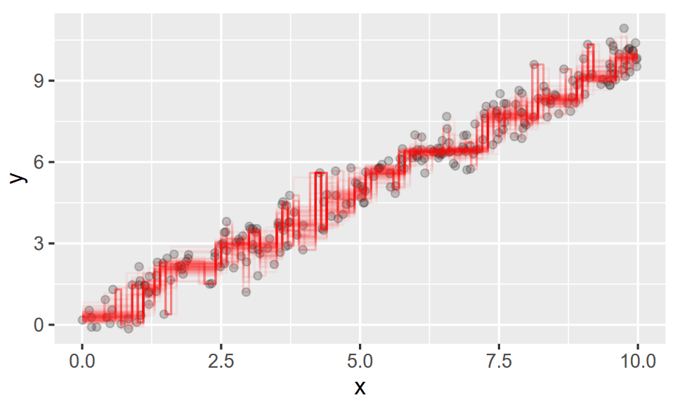
Pruning Trees
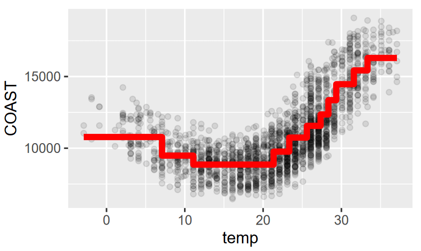
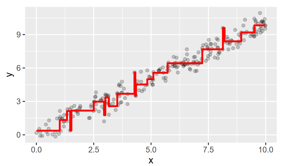
- Trees are always step functions
Pruning Trees
- Trees are always step functions
Pruning Trees
- Trees are always step functions
- They always consider interaction terms and nonlinearities (automatically because each node considers past nodes)
- It also automatically ignore unimportant variables because they never increase fit
- Pros: fast to fit, interpretable, and easily switch between numeric and categorical variables
- Cons: don't scale well, each individual tree can be quite bad at predicting against the testing set
- We'll need to prune!
Pruning Trees
- Grow big:
- Search over each possible splitting rule for the one that gives the biggest increase in fit
- Stop once you reach a minimum threshold (e.g. we only have 10 observations per leaf)
- This is probably overfitted!
- Prune back
- Search over all chosen splits for the one that is the least useful split for goodness of fit
- Stop when you have only a single node
- This has lost most explanatory power!
- But these two processes give a sequence of trees that each of a bias-variance tradeoff that can be cross-validated
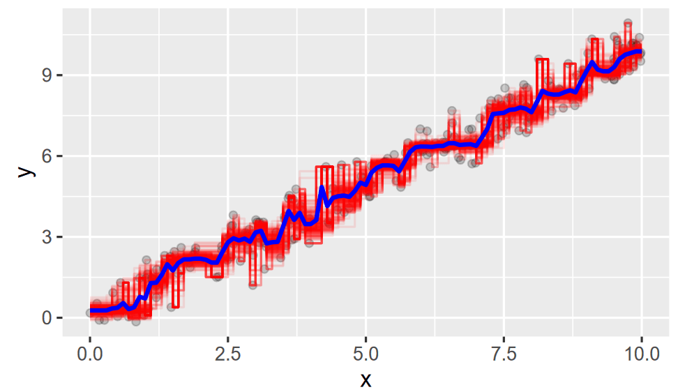
Seeing the Forest
- Bootstrap aggregate ("bagging") over a huge collection of big and pruned trees to get a large selection of trees
- Take the average of those trees and you get the forest
Seeing the Forest
- Bootstrap aggregate ("bagging") over a huge collection of big and pruned trees to get a large selection of trees
- Take the average of those trees and you get the forest
Seeing the Forest
- Bootstrap aggregate ("bagging") over a huge collection of big and pruned trees to get a large selection of trees
- Take the average of those trees and you get the forest
Seeing the Forest
- Bootstrap aggregate ("bagging") over a huge collection of big and pruned trees to get a large selection of trees
- Take the average of those trees and you get the forest
Toy Example

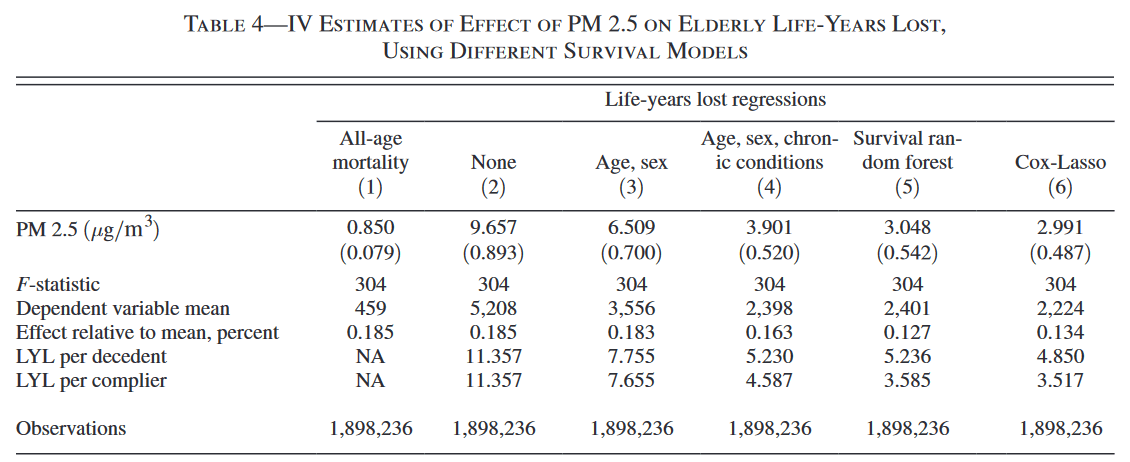
Results
Results
"The richness of our controls suggest this final estimate is about as good a representation of the true value as can be obtained empirically."
Results
"This drop indicates that mortality effects of PM 2.5 tend to be larger among individuals with characteristics that Cox-Lasso associates with lower life expectancy, even after conditioning on age, sex, and chronic conditions."
machine_learning_PM25
By bjw95


