Demand Curves
Christopher Makler
Stanford University Department of Economics
Econ 50: Lecture 9
Demand Curves
Lecture 9
This Week: Graphs
Last Week: Math
Demand curves:
plot demand for one good
in price-quantity space
Offer curves ("consumption loci"):
plot bundles chosen
in good 1-good 2 space
x_1^*(p_1,p_2,m)
x_2^*(p_1,p_2,m)
-
How does \(x_1^*\) change with \(p_1\)?
- Own-price elasticity
- Elastic vs. inelastic
-
How does \(x_1^*\) change with \(p_2\)?
- Cross-price elasticity
- Complements vs. substitutes
-
How does \(x_1^*\) change with \(m\)?
- Income elasticity
- Normal vs. inferior goods
x_1^*(p_1,p_2,m)
Three Relationships
Own-Price Elasticity
What is the effect of a 1% change
in the price of good 1 \((p_1)\) on the quantity demanded of good 1 \((x_1^*)\)?
x_1^*(p_1,p_2,m)
no change
perfectly inelastic
less than 1%
inelastic
exactly 1%
unit elastic
more than 1%
elastic
Cross-Price Elasticity
What is the effect of an increase
in the price of good 2 \((p_2)\) on the quantity demanded of good 1 \((x_1^*)\)?
x_1^*(p_1,p_2,m)
no change
independent
decrease
complements
increase
substitutes
Substitutes
Complements
When the price of one good goes up, demand for the other increases.
When the price of one good goes up, demand for the other decreases.


Income Elasticity
What is the effect of an increase
in income \((m)\) on the quantity demanded of good 1 \((x_1^*)\)?
x_1^*(p_1,p_2,m)
decrease
good 1 is inferior
increase
good 1 is normal
Normal Goods
Inferior Goods
When your income goes up,
demand for the good increases.
When your income goes up,
demand for the good decreases.


Demand Curve for Good 1
Plot relationship
between \(p_1\) and \(x_1^*\),
holding \(p_2\) and \(m\) constant
(ceteris paribus)
Change in \(p_1\): movement along
the demand curve for good 1
x_1^*(p_1,p_2,m)
Change in \(p_2\) or \(m\): shift of
the demand curve for good 1
Procedure
Think about how the behavior
described by the demand function translates into the overall shape of the demand curve:
- Are there discontinuities/cutoff prices where behavior changes?
- What happens as the price gets really high, or approaches zero?
- What fraction of income is being spent on this good?
Choose prices strategically and plot points.
Note: Maximum Possible Quantity Demanded
\overline x_1 = {m \over p_1}

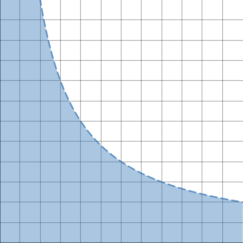

Quantity of Good 1 \((x_1)\)
Price of Good 1 \((p_1)\)
All demand curves must be in this region
Quantity bought at each price if you spent all your money on good 1
x_1 = {m \over p_1}
Leisure-Consumption Tradeoff
Leisure (R)
Consumption (C)
24
24 - L
M
M + \Delta C
You trade \(L\) hours of labor for some amount of consumption, \(\Delta C\).
You start with 24 hours of leisure and \(M\) dollars.
L
\Delta C
You end up consuming \(R = 24 - L\) hours of leisure,
and \(C = M + \Delta C\) dollars worth of consumption.
R
Last Time: MRS, MRT, and the “Gravitational Pull" towards Optimality
Better to produce
more good 1
and less good 2.
MRS
>
MRT
MRS
<
MRT
“Gravitational Pull" Towards Optimality
Better to produce
more good 2
and less good 1.
These forces are always true.
In certain circumstances, optimality occurs where MRS = MRT.
MRS
>
MRT
MRS
<
MRT
Constrained Optimization with One Variable
Think about maximizing each of these functions subject to the constraint \(0 \le x \le 10\).
Pause the video! Try to do these on your own.
Plot the graph on that interval; then find and plot the derivative \(f'(x)\) on that same interval.
Which functions have a maximum at the point where \(f'(x) = 0\)? Why?
f(x) = 5 + 4x - x^2
f(x) = 10 - |2-x|
f(x) = 9 - (x-11)^2
f(x) = 1 + \tfrac{1}{5}(x-5)^2
f(x) = 10 - x
f(x) = 3


Sufficient conditions for an interior optimum characterized by \(f'(x)=0\) with constraint \(x \in [0,10]\)
- \(f'(0) > 0\)
- \(f'(10) < 0\)
- \(f'(x)\) continuous and strictly decreasing on \([0,10]\)
f(x)
f'(x)
x
x
10
0
10
MRS
>
MRT
MRS
<
MRT
Corner Solutions
Interior Solution:
Corner Solution:
Optimal bundle contains
strictly positive quantities of both goods
Optimal bundle contains zero of one good
(spend all resources on the other)
If only consume good 1: \(MRS \ge MRT\) at optimum
If only consume good 2: \(MRS \le MRT\) at optimum
Kinks (Discontinuities)
Kinked Indifference Curve:
Kinked Constraint:
Discontinuities in the MRS
(e.g. Perfect Complements utility function)
Discontinuities in the MRT
(e.g. homework question with two factories)
Monotonicity and Convexity
If preferences are nonmonotonic,
you might be satisfied consuming something within the interior of your feasible set.
FISH
COCONUTS
PPF
If preferences are nonconvex,
the tangency condition might find a minimum rather than a maximum.
FISH
COCONUTS
PPF
Conditions for Calculus to Work
avoids a satiation point within the constraint
At the left corner of the constraint, \(MRS > MRT\)
avoids a corner solution when \(x_1 = 0\)
Monotonicity (more is better)
At the right corner of the constraint, \(MRS < MRT\)
avoids a corner solution when \(x_2 = 0\)
MRS and MRT are continuous as you move along the constraint
avoids a solution at a kink
ensures FOCs find a maximum, not a minimum
Convexity (variety is better)
Unit 1: Scarcity and Choice
Lectures 2 & 3: Derive feasible set (PPF)
from production functions and resource constraints.
Lectures 5 & 6: Solve constrained optimization problem:
find most preferred choice in the feasible set.
Lecture 4: Describe preferences using utility functions.
Unit 2: Consumer Theory
Lecture 7: Derive feasible set (budget set)
as a function of prices and income.
Lectures 9-12: Analyze the comparative statics of how a consumer responds to changes in prices and income.
Lecture 8: Derive the demand function: the optimal bundle as a function of prices and income.
Econ 50 | Fall 2020 | 9 | Demand Curves
By Chris Makler


