Preferences and Utility
To navigate: press "N" to move forward and "P" to move back.
To see an outline, press "ESC". Topics are arranged in columns.
Today's Agenda
Hour 1: Utility Functions
Hour 2: Specific Examples
Quantifying happiness
Indifference Curves as Level Sets
MRS and Marginal Utility
Examples of Utility Functions
Drawing Utility Functions
Equivalent Utility Functions
Chapter 2
Budget Constraints
Chapter 3
Unit Overview
Preferences
Chapter 4
Utility
Chapter 5
Choice
Chapter 6
Demand
Optimization:
Given prices and income, how will a consumer choose to allocate their money?
Comparative Statics:
How do consumers' optimal choices change when prices or income change?
The story so far, in two graphs:
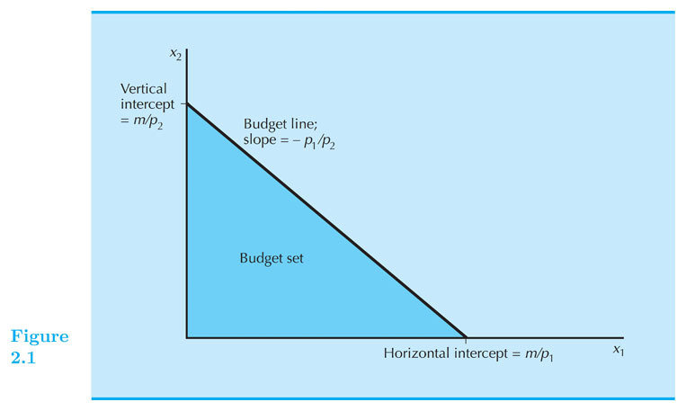
Budget set:
All bundles that cost at most m
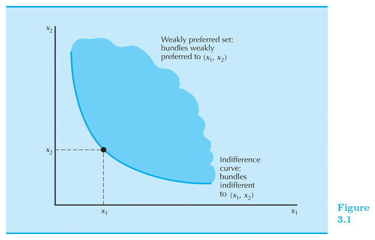
Preferred set:
All bundles that are preferred to X
Goal: find most preferred bundle in the budget set.
Formally: Find a bundle X such that there is no other bundle Y
that is both cheaper than X and preferred to X.
Bringing the Budget Set and Preferred Set Together
Challenge: we have a really good
mathematical description of the budget set;
but we've only discussed preferences in really fuzzy terms.
Topic for today: how do we quantify preferences
in a way that isn't total BS?
Quantifying Happiness
How do I love thee? Let me count the ways.
I love thee to the depth and breadth and height
My soul can reach, when feeling out of sight
For the ends of Being and ideal Grace.
I love thee to the level of everyday’s
Most quiet need, by sun and candlelight.
I love thee freely, as men strive for Right;
I love thee purely, as they turn from Praise.
I love thee with the passion put to use
In my old griefs, and with my childhood’s faith.
I love thee with a love I seemed to lose
With my lost saints,—I love thee with the breath,
Smiles, tears, of all my life!—and, if God choose,
I shall but love thee better after death.
Elizabeth Barrett Browning
Sonnets from the Portugese 43
Utilitarianism
the greatest happiness of the greatest number
is the foundation of morals and legislation.
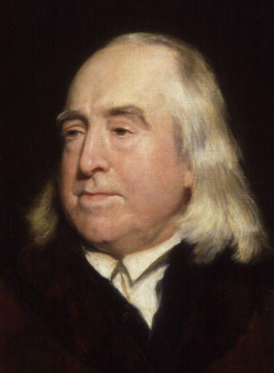
Jeremy Bentham
the utilitarian standard...
is not the agent's own greatest happiness,
but the greatest amount of happiness, altogether.
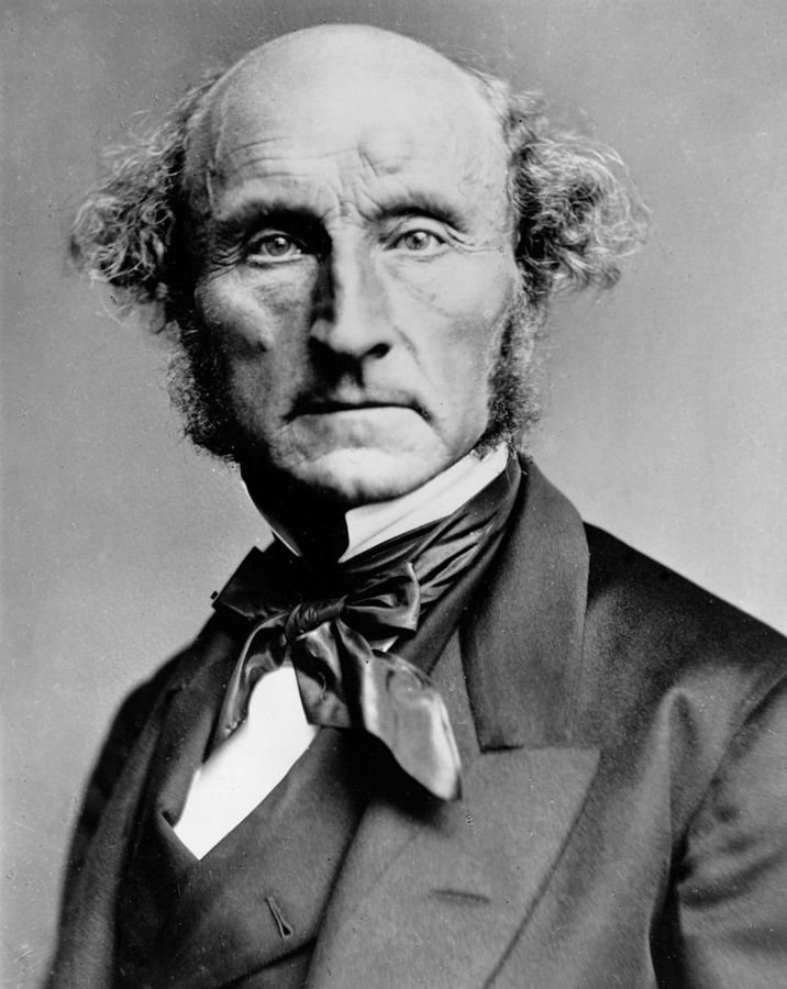
John Stuart Mill
Introduction to the Principles of Morals and Legislation (1789)
Utilitarianism (1861)
Ordinal and Cardinal Preferences
u(a_1,a_2) > u(b_1,b_2)
u(a_1,a_2) \ge u(b_1,b_2)
u(a_1,a_2) = u(b_1,b_2)
u(a_1,a_2) \le u(b_1,b_2)
u(a_1,a_2) < u(b_1,b_2)
u(x_1,x_2)
"A is strictly preferred to B"
Words
Preferences
Utility
A \succ B
A \succeq B
A \sim B
A \preceq B
A \prec B
"A is weakly preferred to B"
"A is indifferent to B"
"A is weakly dispreferred to B"
"A is strictly dispreferred to B"
Suppose the "utility function"
assigns a real number (in "utils")
to every possible consumption bundle
We get completeness because any two numbers can be compared,
and we get transitivity because that's a property of the operator ">"
Plot "utility" as a function.
"Marginal utility" is its derivative.
What could go wrong?


BS METER
What are the units? "Utils?"
All we want to do is to describe
indifference curves and preferred sets mathematically.
Any two "utility functions" that generate the same indifference curves
describe the same preference relation
-- even if the "utility numbers" themselves are nonsense.
Indifference Curves as Level Sets
An indifference curve is a set of all bundles between which a consumer is indifferent.
If a consumer is indifferent between two bundles (A ~ B), then \(u(a_1,a_2) = u(b_1,b_2)\)
Therefore, an indifference curve is a set of all consumption bundles which are assigned the same number of "utils" by the function \(u(x_1,x_2)\)
Likewise, set of bundles preferred to some bundle A is the a set of all consumption bundles which are assigned a greater number of "utils" by \(u(x_1,x_2)\)
u(x_1,x_2) = \sqrt{x_1x_2}
Example: draw the indifference curve for \(u(x_1,x_2) = \frac{1}{2}x_1x_2^2\) passing through (4,6).
Step 1: Evaluate \(u(x_1,x_2)\) at the point
Step 2: Set \(u(x_1,x_2)\) equal to that value.
Step 4: Plug in various values of \(x_1\) and plot!
\(u(4,6) = \frac{1}{2}\times 4 \times 6^2 = 72\)
\(\frac{1}{2}x_1x_2^2 = 72\)
\(x_2^2 = \frac{144}{x}\)
\(x_2 = \frac{12}{\sqrt x_1}\)
How to Draw an Indifference Curve through a Point: Method I
Step 3: Solve for \(x_2\).
How would this have been different if the utility function were \(u(x_1,x_2) = \sqrt{x_1} \times x_2\)?
\(u(4,6) =\sqrt{4} \times 6 = 12\)
\(\sqrt{x_1} \times x_2 = 12\)
\(x_2 = \frac{12}{\sqrt x_1}\)
u(x_1,x_2) = \sqrt{x_1} \times x_2
MRS and Marginal Utility
Marginal Utility
Econ 1: "The additional utility you get from consuming another unit of the good"
Now that we know calculus, it's much easier:
MU_1 = \frac{\partial u(x_1,x_2)}{\partial x_1}
MU_2 = \frac{\partial u(x_1,x_2)}{\partial x_2}
Approximately much additional utility do you get from increasing your consumption of good 1 by 3 units?
What are the units of marginal utility?
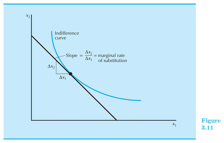
Marginal Rate of Substitution
From last time: "The amount of good 2 you would give up in order to get another unit of good 1 and be no better or worse off"
How much utility do you lose when you give up \(dx_2\) units of good 2?
How much utility do you gain when you get \(dx_1\) units of good 1?
If you gain the same amount of utility from good 1 as you lost from good 2, can you express the MRS in terms of \(dx_1\) and \(dx_2\)?
MRS = \frac{dx_2}{dx_1} = \frac{MU_1}{MU_2}
MRS: Slope of the Indifference Curve
Example: draw the indifference curve for \(u(x_1,x_2) = \frac{1}{2}x_1x_2^2\) passing through (4,6).
Step 1: Derive \(MRS(x_1,x_2)\). Determine its characteristics: is it smoothly decreasing? Constant?
Step 2: Evaluate \(MRS(x_1,x_2)\) at the point.
Step 4: Sketch the right shape of the curve, so that it's tangent to the line at the point.
How to Draw an Indifference Curve through a Point: Method II
Step 3: Draw a line passing through the point with slope \(-MRS(x_1,x_2)\)
How would this have been different if the utility function were \(u(x_1,x_2) = \sqrt{x_1} \times x_2\)?
\text{In both cases }MRS(x_1,x_2) = \frac{MU_1(x_1,x_2)}{MU_2(x_1,x_2)} = \frac{x_2}{2x_1}
MRS(4,6) = \frac{6}{2 \times 4} = \frac{3}{4}
This is continuously strictly decreasing in \(x_1\) and continuously strictly increasing in \(x_2\),
so the function is smooth and strictly convex and has the "normal" shape.
[10 minute break]
Examples of Utility Functions
Perfect Substitutes
Goods that can always be exchanged at a constant rate.
Red pencils and blue pencils, if you con't care about color
One-dollar bills and five-dollar bills
u(x_1,x_2) = ax_1 + bx_2
Exercise 1
For each of these "Perfect Substitute" utility functions, find
the marginal utility with respect to each good,
and then calculate the marginal rate of substitution.
Finally, find an expression for all bundles indifferent to (4,6) and plot it.
u(x_1,x_2) = x_1 + 2x_2
u(x_1,x_2) = \sqrt{x_1 + 2x_2}
u(x_1,x_2) = x_1^2 + 4x_1x_2 + 4x_2^2
u(x_1,x_2) = 4x_1 + 8x_2
u(x_1,x_2) = x_1 + 2x_2 + 4
u(x_1,x_2) = \frac{1}{3}x_1 + \frac{2}{3}x_2
Perfect Complements
Goods that you like to consume
in a constant ratio.
Left shoes and right shoes
Sugar and tea
u(x_1,x_2) = \min \left\{\frac{x_1}{a},\frac{x_2}{b}\right\}
u(x_1,x_2) = \min\{3x_1,x_2\}
Cobb-Douglas
An easy mathematical form with interesting properties.
-
Used for two independent goods (neither complements nor substitutes) -- e.g., t-shirts vs hamburgers
-
Also called "constant shares" for reasons we'll see later.
u(x_1,x_2) = a \ln x_1 + b \ln x_2
u(x_1,x_2) = x_1^ax_2^b
Exercise 2
For each of these Cobb-Douglas utility functions, find
the marginal utility with respect to each good,
and then calculate the marginal rate of substitution.
Finally, find an expression for all bundles indifferent to (4,6) and plot it.
u(x_1,x_2) = x_1x_2^2
u(x_1,x_2) = x_1^{1/3}x_2^{2/3}
u(x_1,x_2) = x_1^{1/10}x_2^{1/5}
u(x_1,x_2) = \frac{1}{2}\ln x_1 + \ln x_2
u(x_1,x_2) = 4x_1x_2^2
u(x_1,x_2) = x_1^{1/2}x_2
u(x_1,x_2) = x_1^\frac{1}{2}x_2
u(x_1,x_2) = x_1^\frac{1}{3}x_2^\frac{2}{3}
u(x_1,x_2) = x_1^ax_2^b
= x_1^\alpha x_2^{1-\alpha} \text{ \ \ for }\alpha = \frac{a}{a+b}
= x_1^\frac{a}{a+b}x_2^\frac{b}{a+b}
\left[x_1^ax_2^b\right]^\frac{1}{a + b}
Handy trick: you can represent any Cobb-Douglas utility function as \(u(x_1,x_2) = x_1^\alpha x_2^{1- \alpha}\)
Quasilinear
Generally used when Good 2 is
"dollars spent on other things."
-
Marginal utility of good 2 is constant
-
If good 2 is "dollars spent on other things," utility from good 1 is often given as if it were in dollars.
\text{e.g., }u(x_1,x_2) = \sqrt x_1 + x_2 \text{ or }u(x_1,x_2) = \ln x_1 + x_2
u(x_1,x_2) = v(x_1) + x_2
u(x_1,x_2) = 10\ln x_1 + x_2
Concave
The opposite of convex: as you consume more of a good, you become more willing to give up others
-
MRS is increasing in \(x_1\) and/or decreasing in \(x_2\)
-
Indifference curves are bowed away from the origin.
e.g., u(x_1,x_2) = ax_1^2 + bx_2^2
u(x_1,x_2) = \left(\frac{x_1}{10}\right)^2 + \left(\frac{x_2}{10}\right)^2
Satiation Point
There is some ideal bundle; utility falls off as you move away from that bundle
-
Not monotonic
-
Realistic, but often the satiation point is far out of reach.
e.g., u(x_1,x_2) = 100 - (x_1 - 10)^2 - (x_2 - 10)^2
"Semi-Satiated"
One good has an ideal quantity; the other doesn't
-
Can be a combination of quasilinear and satiation point
-
Can generate the familiar linear demand curve
e.g., u(x_1,x_2) = 100 - (x_1 - 10)^2 + x_2
We previously had quantitatively defined budget sets
and qualitatively defined preferred sets.
We have now assigned a quantity of "utility" to each
consumption bundle in a way that seems rigorous.
Next step: find the consumption bundle in our budget set that maximizes our utility.
Conclusion and Next Steps
Protip: get to know these utility functions!
They're going to come back over and over again.
Econ 50 | 03 | Preferences and Utility
By Chris Makler
Econ 50 | 03 | Preferences and Utility
The philosophical history of quantifying happiness; some examples of utility functions; indifference curves as level sets (contour lines) of a three-dimensional function; calculating the marginal rate of substitution for utility functions


