Costs in the
Short Run and Long Run
Christopher Makler
Stanford University Department of Economics
Econ 50 : Lecture 15
Today's Agenda
- Review of Econ 1 Treatment of Production and Cost
- Total, Average, and Marginal Costs
- Long-Run Costs and Returns to Scale
- Short-Run Costs and the Marginal Product of Labor
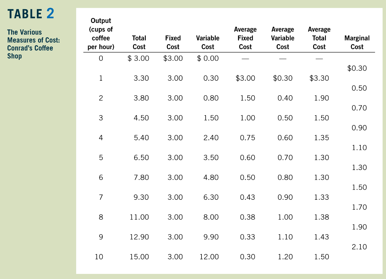
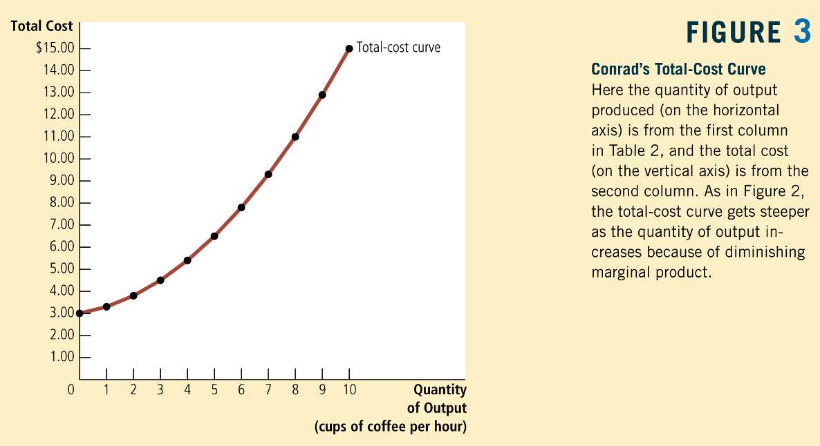
The Econ 1 Approach
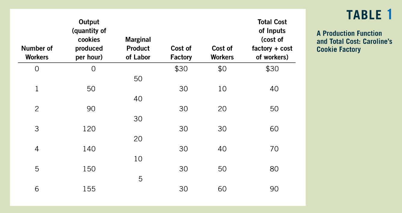
Greg Mankiw, Principles of Economics
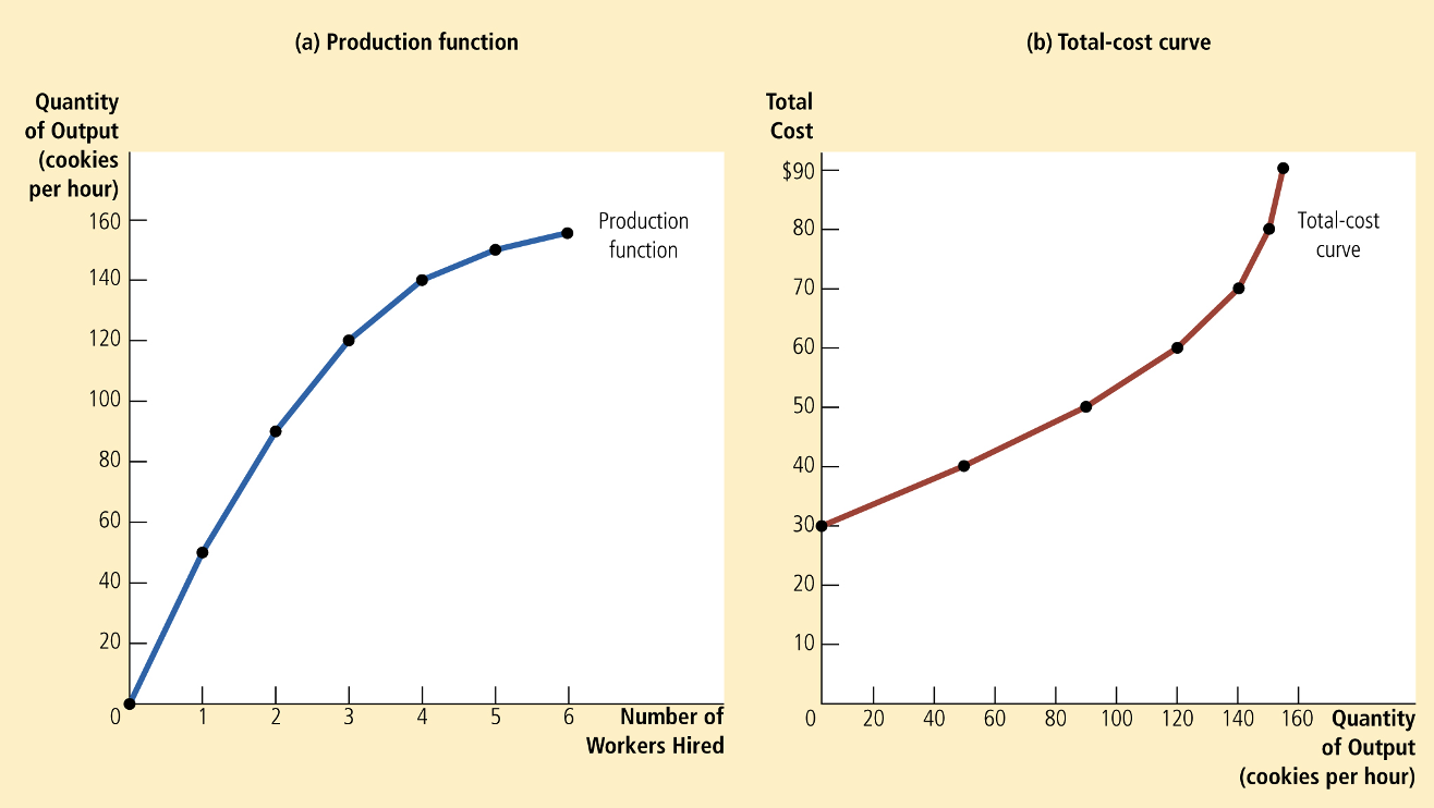
Greg Mankiw, Principles of Economics
Greg Mankiw, Principles of Economics
Greg Mankiw, Principles of Economics
Greg Mankiw, Principles of Economics
Dollars
Dollars Per Unit
Greg Mankiw, Principles of Economics

Total, Average, and Marginal Costs
Total Cost:
c(q) = 100,000
Average Cost:
{c(q) \over q} = {100,000 \over 200} = 500
Marginal Cost:
c'(q) = \text{probably pretty small}

Suppose it costs $100,000 to fly 200 passengers from SFO to NYC
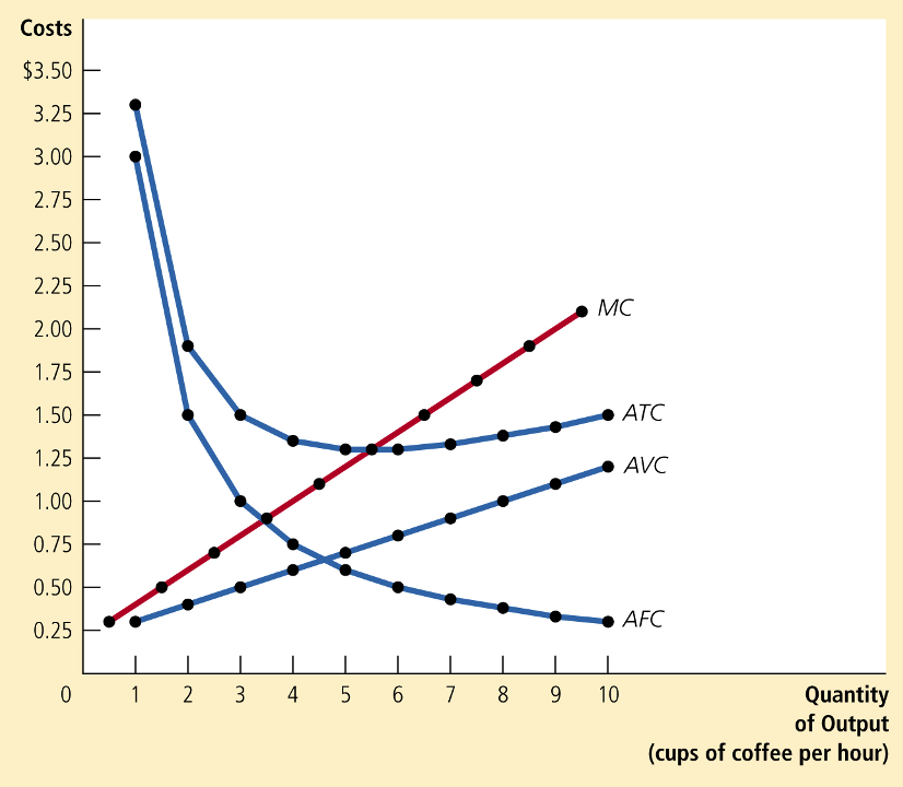
Marginal cost tends to "pull" average cost toward it:
MC > AC \Rightarrow AC \text{ increasing}
MC = AC \Rightarrow AC \text{ constant}
MC < AC \Rightarrow AC \text{ decreasing}
Marginal grade = grade on last test, average grade = GPA
Relationship between Average and Marginal Costs
pollev.com/chrismakler

Suppose q* is the quantity
for which ATC is lowest.
Which of the following must be true?
(Assume that ATC and MC are continuous functions of q.)
(a) MC also reaches its minimum at q*
(b) MC reaches its maximum at q*
(c) MC and ATC are equal at q*
Long-Run Costs
From Last Time: Cost Minimization
Subject to an Output Constraint
\min wL + rK \text{ s.t. } f(L,K) = q
\text{solutions}: L^c(w,r,q), K^c(w,r,q)
Conditional Demand
Expansion Path
A graph connecting the input combinations a firm would use as it expands production: i.e., the solution to the cost minimization problem for various levels of output
Assuming the optimum is found via a tangency condition,
exactly the same as the tangency condition.
Long-Run Total Cost of \(q\) Units
c^{LR}(q) = wL^c(w,r,q) + rK^c(w,r,q)
Conditional demand for labor
Conditional demand for capital
"The total cost of producing \(q\) units in the long run
is the cost of the cost-minimizing combination of inputs
that can produce \(q\) units of output."
L^c(w,r,q)
K^c(w,r,q)
Returns to Scale and Long-Run Cost Functions
From last time: what happens when we increase all inputs proportionally?
For example, what happens if we double both labor and capital?
Does doubling inputs -- i.e., getting \(f(2L,2K)\) -- double output?
f(2L,2K) > 2f(L,K)
f(2L,2K) = 2f(L,K)
f(2L,2K) < 2f(L,K)
Decreasing Returns to Scale
Constant Returns to Scale
Increasing Returns to Scale
f(2L,2K) > 2f(L,K)
f(2L,2K) = 2f(L,K)
f(2L,2K) < 2f(L,K)
Decreasing Returns to Scale
Constant Returns to Scale
Increasing Returns to Scale
pollev.com/chrismakler
When does the production function
f(L,K) = AL^aK^b
exhibit constant returns to scale?
f(L,K)=L^aK^b
Decreasing Returns to Scale
Constant Returns to Scale
Increasing Returns to Scale
f(2L,2K)=(2L)^a(2K)^b
f(2L,2K)=2^{a+b} \times L^aK^b
a + b < 1
2f(L,K)=2 \times L^aK^b
Consider the Cobb-Douglas production function
If we double both labor and capital, we get
How does this compare to double the output?
a + b = 1
a + b > 1
f(L,K)=L^aK^b
Consider the Cobb-Douglas production function
f(L,K)=L^aK^b
\(\theta\) is a constant that depends on \(a\), \(b\), \(w\), and \(r\)...but we're actually just interested in the exponent on \(q\) for right now
The long-run cost function for this is
c(q) = \theta q^{1 \over a + b}
Decreasing Returns to Scale
Constant Returns to Scale
Increasing Returns to Scale
a + b < 1
a + b = 1
a + b > 1
a + b = \tfrac{1}{2} \Rightarrow c(q) = \theta q^2
a + b = 1 \Rightarrow c(q) = \theta q
a + b = 2 \Rightarrow c(q) = \theta q^{1 \over 2}
f(L,K)=L^aK^b
Consider the Cobb-Douglas production function
f(L,K)=L^aK^b
The long-run cost function for this is
c(q) = \theta q^{1 \over a + b}
Decreasing Returns to Scale
Constant Returns to Scale
Increasing Returns to Scale
a + b < 1
a + b = 1
a + b > 1
a + b = \tfrac{1}{2} \Rightarrow c(q) = \theta q^2
a + b = 1 \Rightarrow c(q) = \theta q
a + b = 2 \Rightarrow c(q) = \theta q^{1 \over 2}
- decreasing returns to scale: the long-run total cost curve will get steeper as you produce more output: i.e., you have increasing marginal and average costs.
- If the production function has constant returns to scale, the long-run cost total cost curve will be linear; marginal and average costs are constant.
- increasing returns to scale results in lower costs as you produce more.
Short-Run Costs
Now assume that the level of capital is fixed in the short run at some amount \(\overline K\).
q = f(L\ |\ \overline K)
The amount of labor required to produce \(q\) units of output is therefore also going to depend upon \(\overline K\):
L(q\ |\ \overline K)
Scaling Production in the Short Run
Suppose \(K\) is fixed at some \(\overline K\) in the short run.
Then the production function becomes \(f(L\ |\ \overline K)\)
pollev.com/chrismakler
When does the production function
f(L) = 10L^a
exhibit diminishing marginal product of labor?
Short-Run Expansion Path
- Shows how the firm's choice of labor and capital changes as it expands production.
- If capital is fixed, what does this look like?
Short-Run Total Cost of \(q\) Units
TC(q\ |\ \overline{K}) = wL(q\ |\ \overline{K}) + r\overline{K}
Variable cost
"The total cost of producing \(q\) units in the short run is the variable cost of the required amount of the input that can be varied,
plus the fixed cost of the input that is fixed in the short run."
Fixed cost
f(L,K) = \sqrt{LK}
Short-run conditional demand for labor
if capital is fixed at \(\overline K\):
Total cost of producing \(q\) units of output:
L(q\ |\ \overline K) = {q^2 \over \overline K}
c(q\ |\ \overline{K}) = wL(q\ |\ \overline{K}) + r\overline{K} =
{wq^2 \over \overline K} + r\overline K
Total, Fixed and Variable Costs
c(q\ |\ \overline{K}) =
Fixed Costs \((F)\): All economic costs
that don't vary with output.
Variable Costs \((VC(q))\): All economic costs
that vary with output
explicit costs (\(r \overline K\)) plus
implicit costs like opportunity costs
r\overline{K}
wL(q,\overline{K})
+
TC(q) =
+
F
VC(q)
e.g. cost of labor required to produce
\(q\) units of output given \(\overline K\) units of capital
TC(q) = {wq^2 \over \overline K} + r\overline K
VC(q) = {wq^2 \over \overline K}
F = r\overline K
pollev.com/chrismakler
Generally speaking, if capital is fixed in the short run, then higher levels of capital are associated with _______ fixed costs and _______ variable costs for any particular target output.
\text{Total Cost}: TC(q) = F + VC(q)
\text{Average Cost}: ATC(q) = \frac{TC(q)}{q} = \frac{F}{q} + \frac{VC(q)}{q}
Fixed Costs
Variable Costs
Average Fixed Costs (AFC)
Average Variable Costs (AVC)
Average Costs
\text{Total Cost}: TC(q) = F + VC(q)
\text{Average Cost}: ATC(q) = \frac{F}{q} + \frac{VC(q)}{q}
Average Costs
TC(q) = 64 + {1 \over 4}q^2
ATC(q) = {64 \over q} + {1 \over 4}q
\text{Total Cost}: TC(q) = F + VC(q)
\text{Marginal Cost}: MC(q) = TC'(q) = 0 + VC'(q)
Fixed Costs
Variable Costs
Marginal Cost
(marginal cost is the marginal variable cost)
\text{Total Cost}: TC(q) = F + VC(q)
\text{Marginal Cost}: MC(q) = TC'(q)
Marginal Cost
TC(q) = 64 + {1 \over 4}q^2
MC(q) = {1 \over 2}q
Relationship between Marginal Cost and Marginal Product of Labor
TC(q) = wL^c(q | \overline K) + r \overline K
{dTC(q) \over dq} = w \times {dL^c(q) \over dq}
= w \times {1 \over MP_L}
Comparing the Short Run and the Long Run
Returns to a Single Input
- Increasing marginal product: MPL is increasing in L
- Constant marginal product: MPL is constant in L
- Diminishing marginal product: MPL is decreasing in L
Returns to Scale (Scaling all inputs.)
- Increasing returns to scale: doubling all inputs more than doubles output.
- Constant returns to scale: doubling all inputs exactly doubles output.
- Decreasing returns to scale: doubling all inputs less than doubles output.
f(L,K) = \sqrt{LK}
Long Run (can vary both labor and capital)
L^c(q) = \sqrt{\frac{r}{w}}q
K^c(q) = \sqrt{\frac{w}{r}}q
TC^{LR}(q) = wL^c(q) + rK^c(q)
=2\sqrt{wr}q
Short Run with Capital Fixed at \(\overline K \)
L^c(q | \overline K) = {q^2 \over \overline K}
TC(q) = wL^c(q | \overline K) + r \overline K
={wq^2 \over \overline K} + r \overline K
f(L,K) = \sqrt{LK}
Long Run (can vary both labor and capital)
TC^{LR}(q)=2\sqrt{wr}q
Short Run with Capital Fixed at \(\overline K \)
TC(q)={wq^2 \over \overline K} + r \overline K
Let's fix \(w= 8\), \(r = 2\), and \(\overline K =32\)
TC^{LR}(q)=8q
TC(q)=64 + {1 \over 4}q^2
Relationship between
Short-Run and Long-Run Costs
TC(q | \overline{K}) = \text{Cost if capital is fixed at }\overline{K}
TC(q,K^c(q)) = \text{Cost if capital is fixed at optimal }K \text{ for producing }q
What conclusions can we draw from this?
TC(q,\overline{K}) \ge TC^{LR}(q)
= TC^{LR}(q)
TC^{LR}(q) \text{ is the lower envelope of the family of }TC(q)\text{ curves}
Summary and Next Steps
- Today: derive the long-run and short-run total cost functions and associated unit cost curves for a firm
- Next week: embed this into the profit maximization problem and solve for the optimal output level \(q^*\)
Econ 50 | Fall 25 | Lecture 15
By Chris Makler
Econ 50 | Fall 25 | Lecture 15
Production and Cost for a Firm


