pollev.com/chrismakler

What was Netscape Navigator?
How Markets “Choose" a
Point Along the PPF
Christopher Makler
Stanford University Department of Economics
Econ 50: Lecture 25
Unit IV: Equilibrium
Remaining lectures:
General Equilibrium
Analyze a single market, taking everything determined outside that market as given
(prices of other goods,
consumer income, wages)
Last two lectures:
Partial Equilibrium
Today: examine linkages between markets
Analyze all markets simultaneously
Wednesday: solve for equilibrium quantities in all markets simultaneously as a function only of production functions, resource constraints, and consumer preferences.
(endogenize all prices, income, wages)
Today's Agenda
Labor Markets and the PPF
How Firms Collectively Maximize GDP
Short-Run Supply Response to a Shift in Demand
Review: the PPF and the MRT
Review: Competitive Firms' Demand for Labor
Long-Run Supply Responses and the Long Run Supply Curve
Multiple Uses of Resources
Labor
Fish
🐟
Coconuts
🥥
[GOOD 1]
⏳
[GOOD 2]
Resource Constraint
Resource Constraints and the PPF
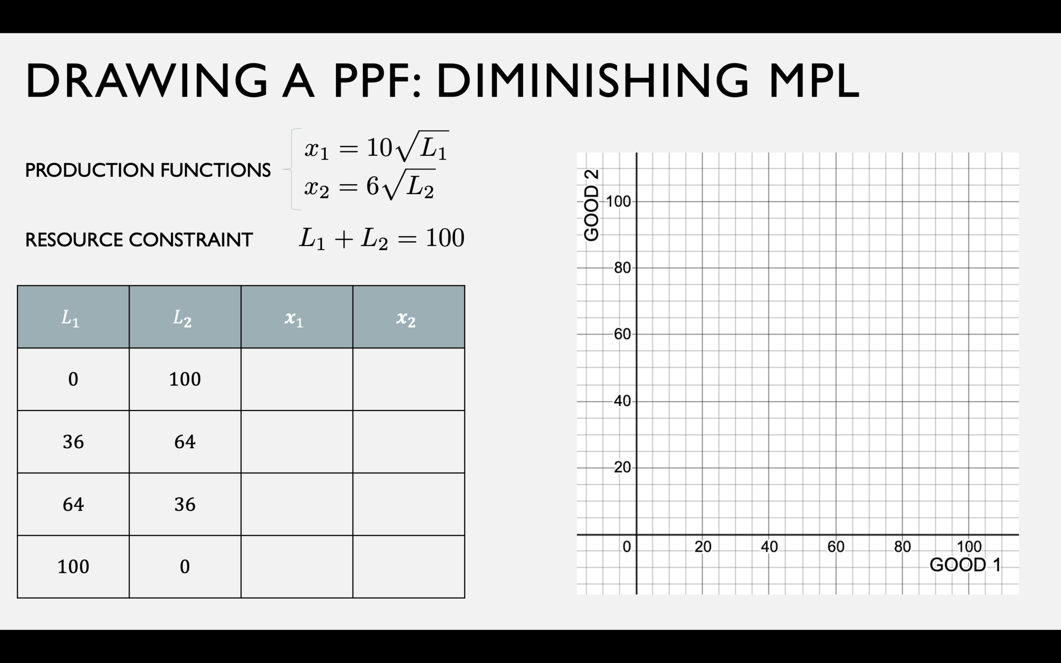

PPF
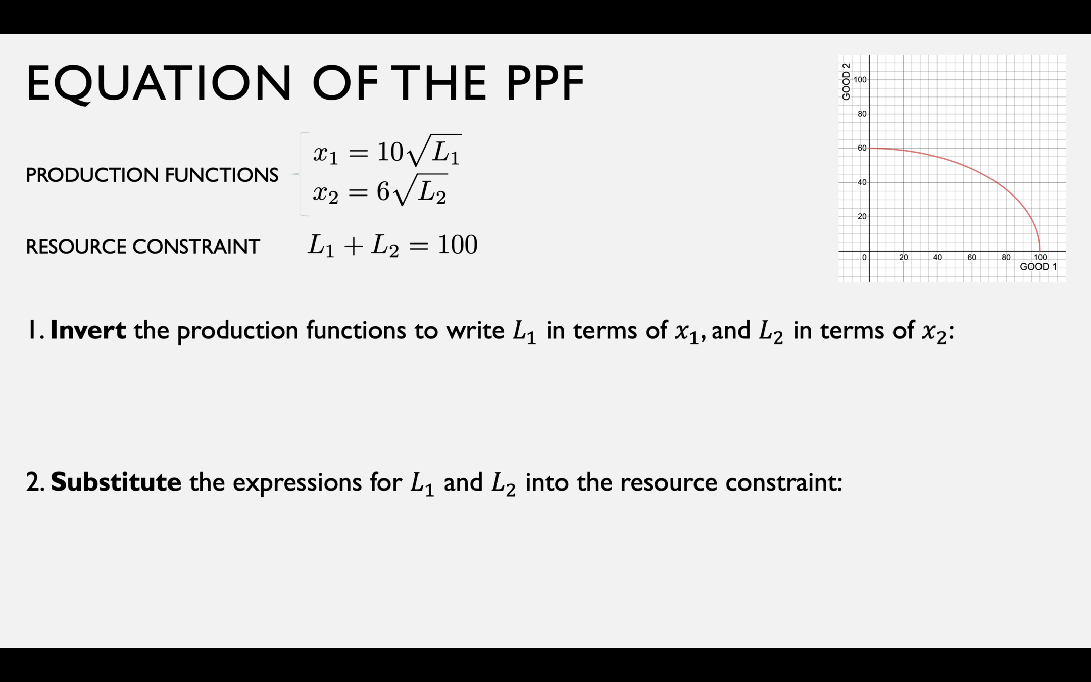

Slope of the PPF:
Marginal Rate of Transformation (MRT)
Rate at which one good may be “transformed" into another
...by reallocating resources from one to the other.
Opportunity cost of producing an additional unit of good 1,
in terms of good 2
Note: we will generally treat this as a positive number
(the magnitude of the slope)
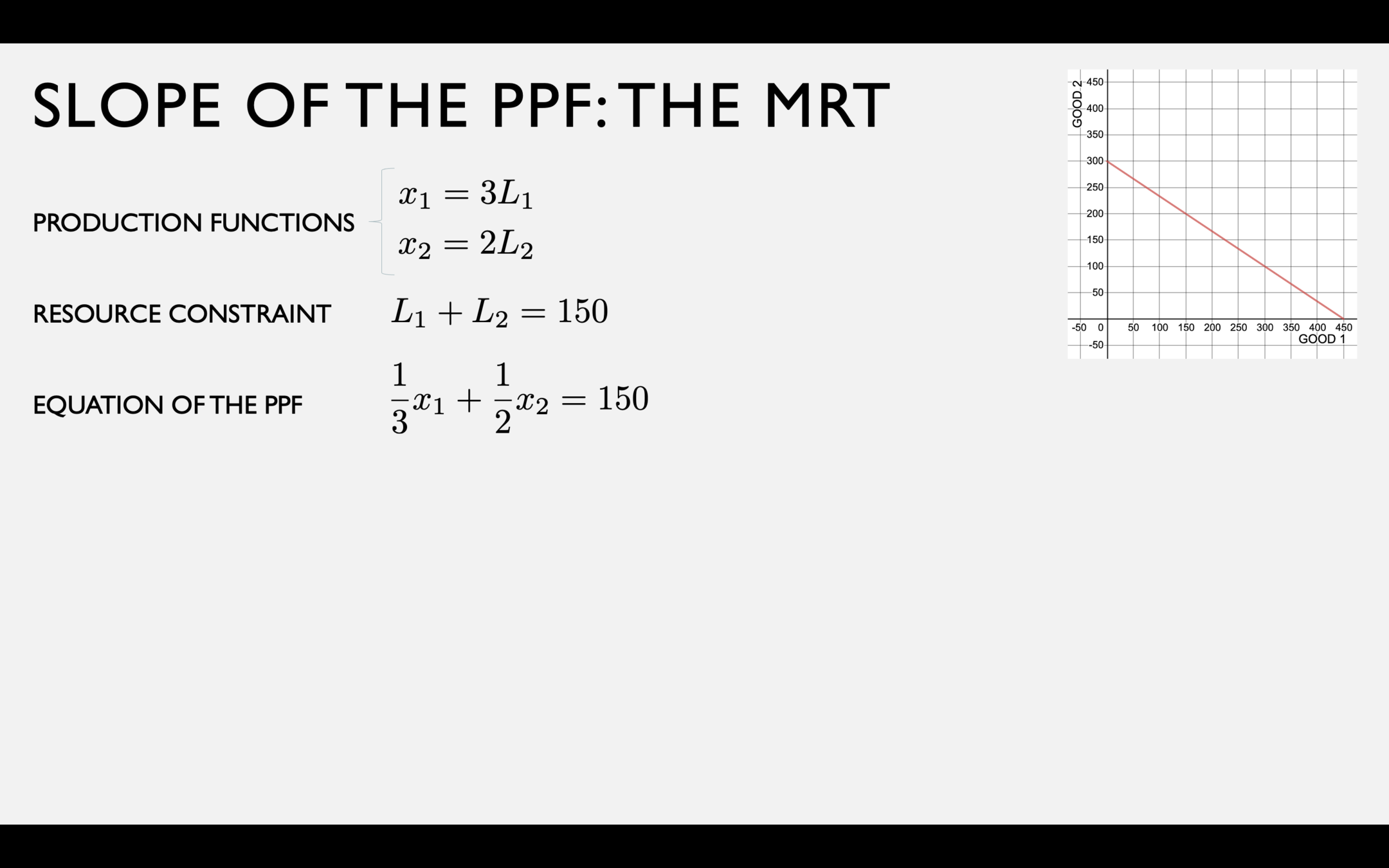
This is just a level set of the function \(L(x_1,x_2) = {1 \over 3}x_1 + {1 \over 2}x_2\)
By the implicit function theorem:

This is just a level set of the function \(L(x_1,x_2) = \)
By the implicit function theorem:
Total labor required to produce the bundle \((x_1,x_2)\)
\(L_1(x_1) + L_2(x_2)\)
\({1 \over 3}x_1 + {1 \over 2}x_2\)
Recall: \(MP_{L1} = {dx_1 \over dL_1}, MP_{L2} = {dx_2 \over dL_2}\)
Suppose we're allocating 100 units of labor to fish (good 1),
and 50 of labor to coconuts (good 2).
Now suppose we shift
one unit of labor
from coconuts to fish.
How many fish do we gain?
100
98
300
303
How many coconuts do we lose?
Relationship between MPL's and MRT
Fish production function
Coconut production function
Resource Constraint
PPF
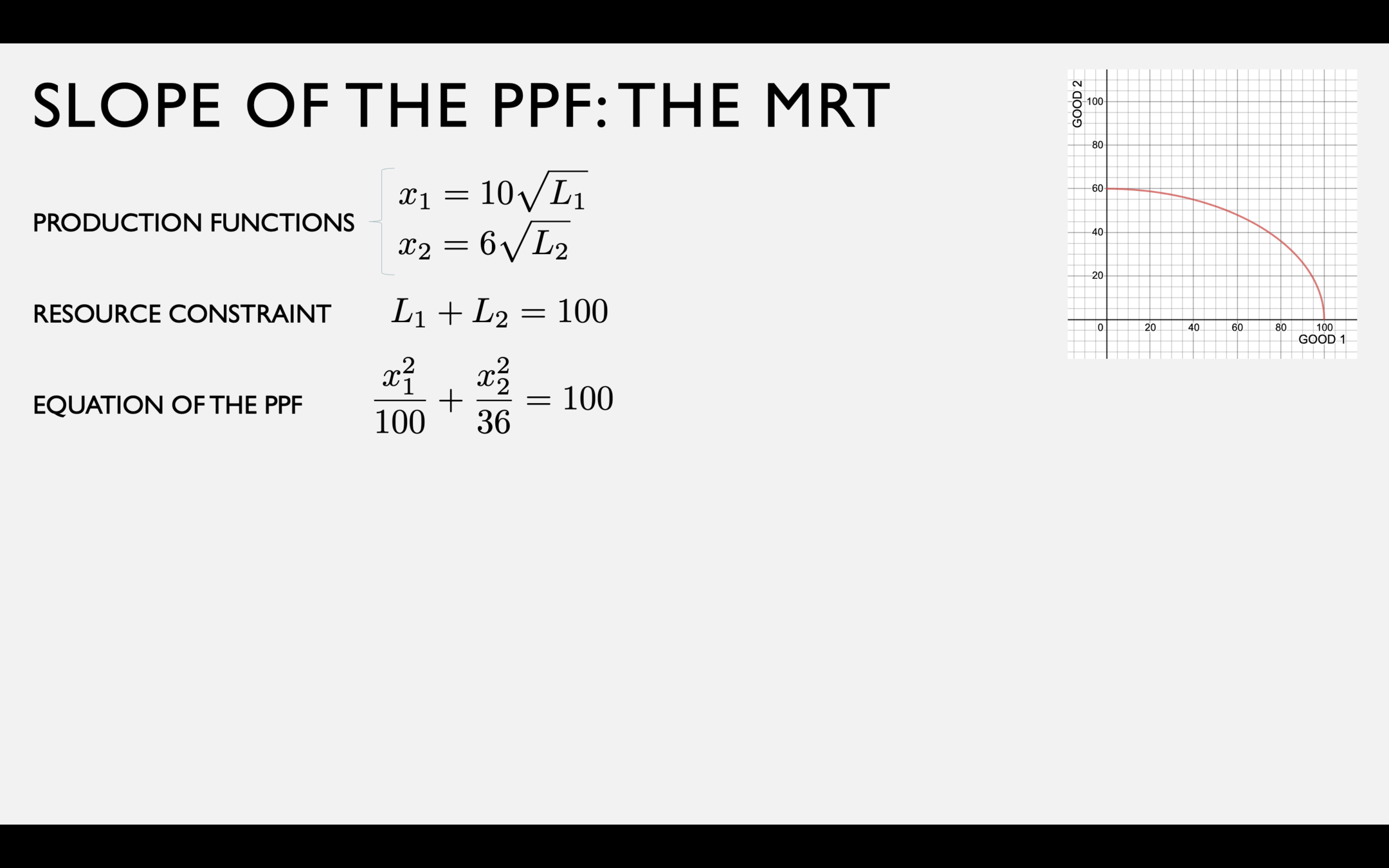
This is a level set of the function \(L(x_1,x_2) = {1 \over 100}x_1^2 + {1 \over 36}x_2^2\)
By the implicit function theorem:
Profit as a function of quantity
Profit as a function of labor
1. Costs and Revenues
2. Profit = total revenues minus total costs
3. Take derivative of profit function, set =0
1. Costs and revenues
2. Profit = total revenues minus total costs
3. Take derivative of profit function, set =0
Profit two ways when \(p = 12\), \(w = 8\), \(r = 2\), and \(\overline K = 32\)
PROFIT-MAXIMIZING OUTPUT CHOICE
PROFIT-MAXIMIZING INPUT CHOICE
When wage is fixed at 8
For a general wage
1. Costs and Revenues
2. Profit = total revenues minus total costs
3. Take derivative of profit function, set =0
Profit-Maximizing Labor Choice when \(p = 12\), \(r = 2\), and \(\overline K = 32\)
NUMBER
FUNCTION
TR
TC
MRPL
MC
Take derivative and set = 0:
Solve for \(L^*\):
PROFIT-MAXIMIZING
LABOR DEMAND FUNCTION
Profit as a function of output \(q\)
Profit as a function of labor \(L\)
1. Costs for general \(w\) and revenue for general \(p\)
2. Profit = total revenues minus total costs
3. Take derivative of profit function, set =0
PROFIT-MAXIMIZING OUTPUT SUPPLY
PROFIT-MAXIMIZING LABOR DEMAND
Profit as a function of output \(q\)
Profit as a function of labor \(L\)
1. Costs for general \(w\) and revenue for general \(p\)
2. Profit = total revenues minus total costs
3. Take derivative of profit function, set =0
[cost of labor required for \(q\) units of output]
[revenue of output produced by \(L\) hours of labor]
MARGINAL COST (MC)
MARGINAL REVENUE PRODUCT OF LABOR (MRPL)
"Keep producing output as long as the marginal revenue from the last unit produced is at least as great as the marginal cost of producing it."
"Keep hiring workers as long as the marginal revenue from the output of the last worker is at least as great as the cost of hiring them."
Profit as a function of output \(q\)
Profit as a function of labor \(L\)
Labor Markets and the PPF
Notation
\(Y_1\) = total amount of good 1 produced by all firms in an economy
\(Y_2\) = total amount of good 2 produced by all firms in an economy
\(GDP(Y_1,Y_2) = p_1Y_1 + p_2Y_2\)
= market value of all final goods and services produced in an economy
Recall: market demand for a good is the horizontal sum of all individual demand curves:
The same is true for labor demand!
What happens to the individual and market labor demand when the price of good 1 goes up?
Let's do the math!
Suppose for simplicity that each good is produced by a single competitive firm.
Total labor demanded is the sum of the labor demanded by each firm, at any wage:
Suppose that labor is supplied inelastically at \(\overline L = 100\).
We can solve for the equilibrium wage rate by equating labor demand and supply:
What happens to the individual and market labor demand when the price of good 1 goes up?
So, how does this affect output?
How Firms Collectively Maximize GDP
Resource Allocation
Narrow question:
How many productive resources should we devote to a single good?
Broader question:
How should we allocate productive resources across goods?
Firms will choose the quantity at which \(p = MC\)
Firms will choose the point along the PPF at which \({p_1 \over p_2} = MRT\)
GDP maximizing point!!
How do firms
maximize GDP?
For a given set of prices \((p_1,p_2)\), what combination of outputs \((Y_1,Y_2)\) on our PDF would maximize GDP?
\(GDP(Y_1,Y_2) = p_1Y_1 + p_2Y_2\)
(Assume labor is the only input.)
pollev.com/chrismakler

What is the magnitude of the slope of an iso-GDP line?
The Social Planner's Problem
How do we maximize GDP subject to the PPF?
OBJECTIVE
FUNCTION
CONSTRAINT
DOLLARS
HOURS
What are the units?
DOLLARS
PER
HOUR
FIRST ORDER CONDITIONS
Tangency condition:
Firms setting their own MRPL equal to the wage rate will choose the point along the PPF at which \({p_1 \over p_2} = MRT\)
Conditions for
GDP Maximization
TANGENCY CONDITION
CONSTRAINT CONDITION
Firms in industry 1 set \(w = p_1 \times MP_{L1}\)
Firms in industry 2 set \(w = p_2 \times MP_{L2}\)
How does competition achieve this?
Wages adjust until the
labor market clears

Effect of a Change in Demand
Consider two goods (“guns” and “butter”) which are unrelated
but which both use the same resource (e.g. labor) in production.
What happens in both markets
if there is a demand shift
in the market for one of the goods?
pollev.com/chrismakler

Why did the wage rate go up in this model?
“Chain of Causality"
- Increase in demand for good 1:
- Movement up along the supply curve for good 1 → produce more good 1, increase \(p_1\)
- Increase \(p_1\) → outward shift of the demand for labor from firms producing good 1
- Increase in labor demand → equilibrium wage increases for all firms
- Increase in wage affects supply of good 2:
- Movement up along the labor demand curve for firms producing good 2
- Inward shift of the supply curve for good 2 → produce less good 2
- Secondary effect: increase in wage also reduces supply of good 1
- Cumulative effect:
- Produce more good 1 and less 2.
- Use same amount of labor in total → stay along the PPF
Econ 50 | Lecture 25
By Chris Makler
Econ 50 | Lecture 25
Relationships Between Markets
- 931


