Nash Equilibrium
Christopher Makler
Stanford University Department of Economics
Econ 51: Lecture 4
- Part I: Pure strategies
- Part II: Mixed strategies
- Part III: Continuous strategies
Today's Agenda
Best Response: The Slide I Should Have Put Up Last Time
\text{Let }\theta_{-i}\text{ be player }i\text{'s beliefs about the strategies}
\text{We say }s_{i}\text{ is a \textbf{best response} given }\theta_{-i}\text{ if}
u_i(s_i,\theta_{-i}) \ge u_i(s'_i,\theta_{-i})
\text{ for every available strategy }s'_i \in S_i
In plain English: given my beliefs about what the other player(s) are doing, a strategy is my "best response"
if there is no other strategy available to me
that would give me a higher payoff.
\text{ player }i\text{'s payoff from }s_i
\text{ player }i\text{'s payoff from }s'_i
\text{being played by all players other than player }i
Best Response under Strategic Certainty
\text{Let }s_{-i}\text{ be the strategies being played by all players other than player }i
\text{We say }s_{i}^*\text{ is a \textbf{best response} to }s_{-i}\text{ if}
u_i(s_i^*,s_{-i}) \ge u_i(s'_i,s_{-i})
\text{ for every available strategy }s'_i \in S_i
In plain English: given the strategies chosen by the other player(s),
a strategy is my "best response"
if there is no other strategy available to me
that would give me a higher payoff.
\text{ player }i\text{'s payoff from }s_i^*
\text{ player }i\text{'s payoff from }s'_i
Possible rationales for strategic certainty:
- People play this game all the time, and reasonably expect
the other player to play according to the equilibrium. - The players have agreed on a strategy before the game is played;
as long as no one has an incentive to deviate, it's OK. - An outside mediator (society, the law) recommends a strategy profile
Stag Hunt Game
1
2
Stag
Hare
Stag
Hare
5
5
,
4
0
,
4
4
,
0
4
,

Equilibrium
Definition: Best Response (Nash) Equilibrium
\text{A strategy profile }s^* = s_1^*,s_2^*,...,s^*_n\text{ is a \textbf{Nash Equilibrium} if}
u_i(s^*) \ge u_i(s'_i,s^*_{-i})
\text{ for every available strategy }s'_i \in S_i \text{, for all players } i=1,2,...,n
In plain English: in a Nash Equilibrium, every player is playing a best response to the strategies played by the other players.
\text{ player }i\text{'s equilibrium payoff}
\text{ player }i\text{'s payoff from some deviation }s'_i
In other words: there is no profitable unilateral deviation
given the other players' equilibrium strategies.
Coordination Game
1
2
Opera
Movie
Opera
Movie
2
1
,
0
0
,
1
2
,
0
0
,
pollev.com/chrismakler

Pareto Coordination
1
2
A
B
A
B
2
2
,
0
0
,
1
1
,
0
0
,
pollev.com/chrismakler
Matching Pennies I: Coordination Game
1
2
Heads
Tails
Heads
Tails
1
1
,
-1
-1
,
1
1
,
-1
-1
,
Each player chooses Heads or Tails.
If they choose the same thing,
they both "win" (get a payoff of 1).
If they choose differently,
they both "lose" (get a payoff of -1).
Circle best responses.
What are the Nash equilibria of this game?
Matching Pennies II: Zero-Sum Game
1
2
Heads
Tails
Heads
Tails
1
-1
,
-1
1
,
1
-1
,
-1
1
,
Each player chooses Heads or Tails.
If they choose the same thing,
player 1 "wins" (gets a payoff of 1)
and player 2 "loses" (gets a payoff of -1).
If they choose differently,
they player 1 "loses" (gets a payoff of -1)
and player 1 "wins" (gets a payoff of 1).
Circle best responses.
What are the Nash equilibria of this game?
Best Response
If two or more pure strategies are best responses given what the other player is doing, then any mixed strategy which puts probability on those strategies (and no others) is also a best response.
2
\({1 \over 6}\)
\({1 \over 3}\)
\({1 \over 2}\)
\(0\)
Player 2's strategy
\({1 \over 6} \times 6 + {1 \over 3} \times 3 + {1 \over 2} \times 2 + 0 \times 7\)
\(=3\)
\({1 \over 6} \times 12 + {1 \over 3} \times 6 + {1 \over 2} \times 0 + 0 \times 5\)
\(=4\)
\({1 \over 6} \times 6 + {1 \over 3} \times 0 + {1 \over 2} \times 6 + 0 \times 11\)
\(=4\)
Player 1's expected payoffs from each of their strategies
\(X\)
\(A\)
1
\(B\)
\(C\)
\(D\)
\(Y\)
\(Z\)
6
6
,
3
6
,
2
8
,
7
0
,
12
6
,
6
3
,
0
2
,
5
0
,
6
0
,
0
9
,
6
8
,
11
4
,
If player 2 is choosing this strategy, player 1's best response is to play either Y or Z.
Therefore, player 1 could also choose to play any mixed strategy \((0, p, 1-p)\).
When is a mixed strategy a best response?
1
2
Heads
Tails
Heads
Tails
1
-1
,
-1
1
,
1
-1
,
-1
1
,
Let's return to our zero-sum game.
\((p)\)
\((1-p)\)
What is player 1's expected payoff from Heads?
Suppose player 2 is playing a mixed strategy: Heads with probability \(p\),
and tails with probability \(1-p\).
What is player 1's expected payoff from Tails?
1 \times p + -1 \times (1-p)
= 2p - 1
-1 \times p + 1 \times (1-p)
= 1 - 2p
For what value of \(p\) would player 1 be willing to mix?
2p - 1 = 1 - 2p
\Rightarrow p = {1 \over 2}
When is a mixed strategy a best response?
1
2
Heads
Tails
Heads
Tails
1
-1
,
-1
1
,
1
-1
,
-1
1
,
\((p)\)
\((1-p)\)
For what value of \(p\) would player 1 be willing to mix?
p = {1 \over 2}
Now suppose player 1 does mix, and plays Heads with probability \(q\) and Tails with probability \(1 - q\).
\((q)\)
\((1-q)\)
For what value of \(q\) would player 2 be willing to mix?
\text{By the same logic, }q = {1 \over 2}
Equilibrium in Mixed Strategies
A mixed strategy profile is a Nash equilibrium if,
given all players' strategies, each player is mixing among strategies which are their best responses
(i.e. between which they are indifferent)
Important: nobody is trying to make the other player(s) indifferent; it's just that in equilibrium they are indifferent.
Oligopoly
Applications of Game Theory:
Strategic Interactions between Small Numbers of Agents
- Very realistic - lots of examples, from families to international diplomacy
- Models of oligopoly
- 1838: Cournot
- 1883: Bertrand
- 1929: Hotelling
- 1934: Stackelberg
- Mid-20th century: John Nash formalized and generalized the notion of strategic equilibrium among small numbers of agents
- We will follow this intellectual history, by first analyzing oligopoly models and then generalizing to look at broader classes of problems
Competition
- Lots of "small" firms selling basically the same thing (commodity goods)
Oligopoly
- A few "medium" or "large" firms selling differentiated products
- Firms face essentially horizontal demand curve
- Firms face downward sloping demand curve
-
Interdependence:
each firm's choice
affects other firms
-
Independence:
no individual firm's choice affects other firms


Review: Monopoly
Simple case: linear demand, constant MC, no fixed costs
P(Q) = 14 - Q
c(Q) = 2Q
\text{No fixed costs }\Rightarrow MC = AC = 2
Baseline Example: Monopoly
P(Q) = 14 - Q
c(Q) = 2Q
\pi(Q) = P(Q)Q - c(Q)
= (14 - Q)Q - 2Q
= 14Q - Q^2 - 2Q
\text{total revenue}
\text{total cost}
14
2
units
$/unit
P(Q) = 14 - Q
MC = AC = 2
\text{No fixed costs }\Rightarrow MC = AC = 2
14
P
Q
Baseline Example: Monopoly
P(Q) = 14 - Q
c(Q) = 2Q
\pi(Q) = P(Q)Q - c(Q)
= (14 - Q)Q - 2Q
= 14Q - Q^2 - 2Q
\text{total revenue}
\text{total cost}
14
2
units
$/unit
P(Q) = 14 - Q
MC = AC = 2
\text{No fixed costs }\Rightarrow MC = AC = 2
14
P
Q
Profit
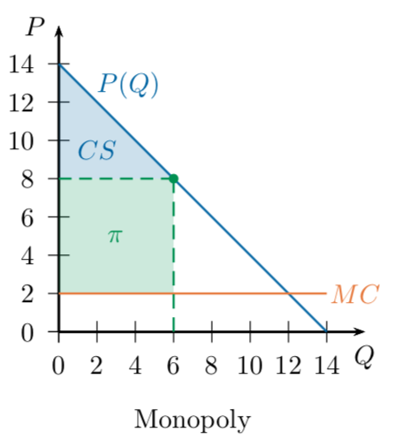
Baseline Example: Monopoly
P(Q) = 14 - Q
c(Q) = 2Q
\pi(Q) = P(Q)Q - c(Q)
= (14 - Q)Q - 2Q
= 14Q - Q^2 - 2Q
\pi'(Q) = 14 - 2Q - 2 = 0
Q^* = 6
\text{total revenue}
\text{total cost}
\text{marginal revenue}
\text{marginal cost}
P^* = 14 - 6 = 8
\pi^* = 8\times 6 - 2 \times 6 = 36
14
8
2
6
Q
P
P(Q) = 14 - Q
MR(Q) = 14 - 2Q
MC = AC = 2
36
Duopoly
Quantity Duopoly
- Two firms ("duo" in duopoly)
- Each chooses how much to produce
- Market price depends on
the total amount produced - Each firm faces a residual demand curve
based on the other firm's choice
What is firm 2's best response function?
P(q_1,q_2) = 14 - (q_1+q_2)
c_2(q_2) = 2q_2
\pi_2(q_2) = P(q_1 + q_2)q_2 - c_2(q_2)
= (14 - q_1 - q_2)q_2 - 2q_2
= 14q_2 - q_1q_2 - q_2^2 - 2q_2
\pi'_2(q_2) = 14-q_1 - 2q_2 - 2 = 0
q_2^*(q_1) = 6-\frac{1}{2}q_1
\text{total revenue}
\text{total cost}
\text{marginal revenue}
\text{marginal cost}
2
P
P(q_2|q_1) = 14-q_1 - q_2
MR(Q) = 14-q_1 - 2q_2
MC(q_2) = 2
6-\frac{1}{2}q_1
14-q_1
q_2
"Firm 2's Residual Demand Curve"
Firm 2's "best response function"
Cournot Model:
Both firms choose simultaneously and independently
q_1^*(\hat q_2) = 6 - {1 \over 2}\hat q_2
Firm 1's
best response function
q_2^*(\hat q_1) = 6 - {1 \over 2}\hat q_1
Firm 2's
best response function
In equilibrium, each firm is
correct in its beliefs (so \(q_1 = \hat q_1\) and \(q_2 = \hat q_2\) ),
so each firm's quantity is a best response to the other firm's quantity.
q_1
q_2
q_1^*(\hat q_2) = 6 - {1 \over 2}\hat q_2
q_2^*(\hat q_1) = 6 - {1 \over 2}\hat q_1
q_1
q_2
q_1^*(\hat q_2) = 6 - {1 \over 2}\hat q_2
q_2^*(\hat q_1) = 6 - {1 \over 2}\hat q_1
Another way of thinking about this:
if everyone knows everything about this model (and everyone knows that everyone knows everything about this model), what do each of the firms know about the other firm's beliefs?
Each firm knows the other
will never produce more than 6.
Because \(6 - {1 \over 2}6 = 3\),
this means each firm knows the other
will never produce less than 3.
Because \(6 - {1 \over 2}3 = 4.5\),
this means each firm knows the other
will never produce more than 4.5.
The only set of quantities that survives this is (4,4).
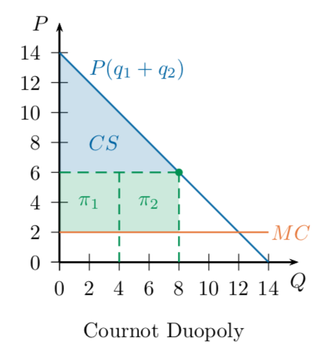
Profits in Cournot Equilibrium
Each firm is producing 4 units, so the market price is \(14 - 4 - 4 = 6\).
Each unit costs $2, so each firm is making
$4 of profit on 4 units = $16.
Remember our monopoly: it produced 6 units,
sold them at a price of 8, and earned a total profit of 36.
If each of these two firms produced 3 units, they could earn 18...
so why don't they?
Next Thursday, we'll look at collusion between firms.
Next Week
- How does introducing time affect the kinds of outcomes we can observe in equilibrium?
Econ 51 | Spring 23 | 4 | Nash Equilibrium
By Chris Makler
Econ 51 | Spring 23 | 4 | Nash Equilibrium
Introduction to game theory; dominance and best response; Nash equilibrium


