Oligopoly
Christopher Makler
Stanford University Department of Economics
Econ 51: Lecture 12
Applications of Game Theory:
Strategic Interactions between Small Numbers of Agents
- Very realistic - lots of examples, from families to international diplomacy
- Models of oligopoly
- 1838: Cournot
- 1883: Bertrand
- 1929: Hotelling
- 1934: Stackelberg
- Mid-20th century: John Nash formalized and generalized the notion of strategic equilibrium among small numbers of agents
- We will follow this intellectual history, by first analyzing oligopoly models and then generalizing to look at broader classes of problems
Competition
- Lots of "small" firms selling basically the same thing (commodity goods)
Oligopoly
- A few "medium" or "large" firms selling differentiated products
- Firms face essentially horizontal demand curve
- Firms face downward sloping demand curve
-
Interdependence:
each firm's choice
affects other firms
-
Independence:
no individual firm's choice affects other firms


If you're interested in this stuff..
Today's Agenda
- Establish two basic models:
- Model 1 (Cournot): Firms choose quantities,
market price is determined by those choices - Model 2 (Hotelling): Firms choose prices,
quantities sold by each firm are determined by those choices
- Model 1 (Cournot): Firms choose quantities,
- Today: simultaneous choice games.
- Next week: introduce timing
- Week after: introduce private information
Review: Monopoly
Simple case: linear demand, constant MC, no fixed costs
P(Q) = 14 - Q
c(Q) = 2Q
\text{No fixed costs }\Rightarrow MC = AC = 2
Baseline Example: Monopoly
P(Q) = 14 - Q
c(Q) = 2Q
\pi(Q) = P(Q)Q - c(Q)
= (14 - Q)Q - 2Q
= 14Q - Q^2 - 2Q
\text{total revenue}
\text{total cost}
14
2
units
$/unit
P(Q) = 14 - Q
MC = AC = 2
\text{No fixed costs }\Rightarrow MC = AC = 2
14
P
Q
Baseline Example: Monopoly
P(Q) = 14 - Q
c(Q) = 2Q
\pi(Q) = P(Q)Q - c(Q)
= (14 - Q)Q - 2Q
= 14Q - Q^2 - 2Q
\text{total revenue}
\text{total cost}
14
2
units
$/unit
P(Q) = 14 - Q
MC = AC = 2
\text{No fixed costs }\Rightarrow MC = AC = 2
14
P
Q
Profit
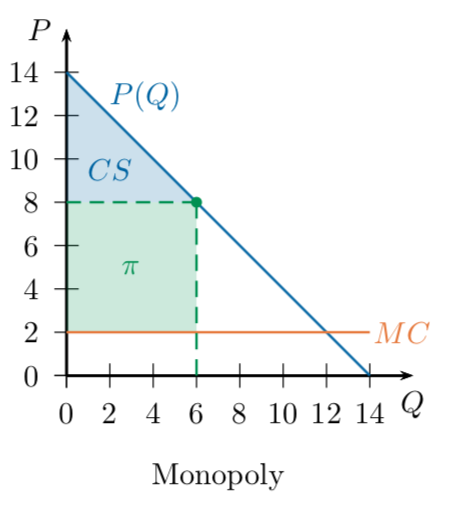
Baseline Example: Monopoly
P(Q) = 14 - Q
c(Q) = 2Q
\pi(Q) = P(Q)Q - c(Q)
= (14 - Q)Q - 2Q
= 14Q - Q^2 - 2Q
\pi'(Q) = 14 - 2Q - 2 = 0
Q^* = 6
\text{total revenue}
\text{total cost}
\text{marginal revenue}
\text{marginal cost}
P^* = 14 - 6 = 8
\pi^* = 8\times 6 - 2 \times 6 = 36
14
8
2
6
Q
P
P(Q) = 14 - Q
MR(Q) = 14 - 2Q
MC = AC = 2
36
Cournot Duopoly
Cournot Duopoly
- Two firms ("duo" in duopoly)
- Each chooses how much to produce (quantity competition)
- Market price depends on the total amount produced
- Each firm faces a residual demand curve
based on the other firm's choice
What is firm 2's best response function?
P(q_1,q_2) = 14 - (q_1+q_2)
c_2(q_2) = 2q_2
\pi_2(q_2) = P(q_1 + q_2)q_2 - c_2(q_2)
= (14 - q_1 - q_2)q_2 - 2q_2
= 14q_2 - q_1q_2 - q_2^2 - 2q_2
\pi'_2(q_2) = 14-q_1 - 2q_2 - 2 = 0
q_2^*(q_1) = 6-\frac{1}{2}q_1
\text{total revenue}
\text{total cost}
\text{marginal revenue}
\text{marginal cost}
2
P
P(q_2|q_1) = 14-q_1 - q_2
MR(Q) = 14-q_1 - 2q_2
MC(q_2) = 2
6-\frac{1}{2}q_1
14-q_1
q_2
"Firm 2's Residual Demand Curve"
Firm 2's "best response function"
Cournot Model:
Both firms choose simultaneously and independently
q_1^*(\hat q_2) = 6 - {1 \over 2}\hat q_2
Firm 1's
best response function
q_2^*(\hat q_1) = 6 - {1 \over 2}\hat q_1
Firm 2's
best response function
In equilibrium, each firm is
correct in its beliefs (so \(q_1 = \hat q_1\) and \(q_2 = \hat q_2\) ),
so each firm's quantity is a best response to the other firm's quantity.
q_1
q_2
q_1^*(\hat q_2) = 6 - {1 \over 2}\hat q_2
q_2^*(\hat q_1) = 6 - {1 \over 2}\hat q_1
q_1
q_2
q_1^*(\hat q_2) = 6 - {1 \over 2}\hat q_2
q_2^*(\hat q_1) = 6 - {1 \over 2}\hat q_1
Another way of thinking about this:
if everyone knows everything about this model (and everyone knows that everyone knows everything about this model), what do each of the firms know about the other firm's beliefs?
Each firm knows the other
will never produce more than 6.
Because \(6 - {1 \over 2}6 = 3\),
this means each firm knows the other
will never produce less than 3.
Because \(6 - {1 \over 2}3 = 4.5\),
this means each firm knows the other
will never produce more than 4.5.
The only set of quantities that survives this is (4,4).
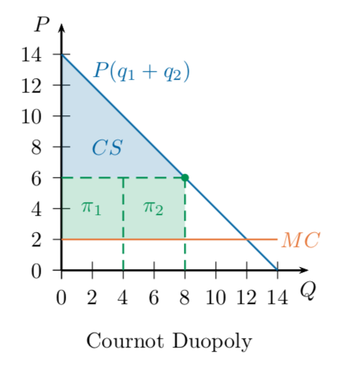
Profits in Cournot Equilibrium
Each firm is producing 4 units, so the market price is \(14 - 4 - 4 = 6\).
Each unit costs $2, so each firm is making
$4 of profit on 4 units = $16.
Remember our monopoly: it produced 6 units,
sold them at a price of 8, and earned a total profit of 36.
If each of these two firms produced 3 units, they could earn 18...
so why don't they?
Next Thursday, we'll look at collusion between firms.
Hotelling Duopoly
Hotelling Duopoly
- Two stores, located at different points along a "street"
- Selling the same product, but consumers incur a travel cost c per distance traveled to the store
- Each chooses how much to charge (price competition)
- Market shares are determined by the indifferent consumer
- As before, each store faces a residual demand curve based on the other store's choice
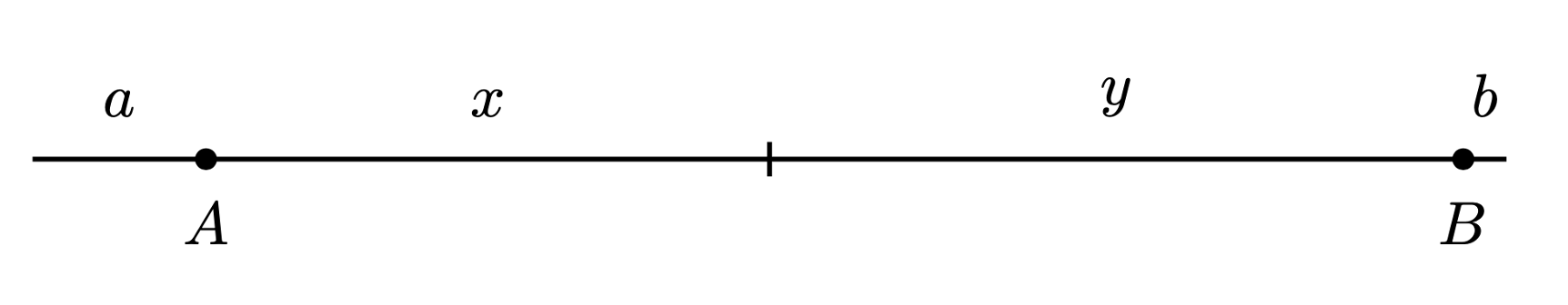
- Stores A and B are located along a street of length \(l\)
- Store A is \(a\) blocks from one end, store B is \(b\) blocks from the other.
- They sell the same products; only differentiator is location.
- Assume no costs to either store; they’re just trying to maximize revenue.
- Consumers are uniformly distributed along the street.
\ l\
\ l\
🤓
Indy
Indy is located \(x\) blocks from store A, and \(y\) blocks from store B.
\ l\
🤓
Indy
Indy is located \(x\) blocks from store A, and \(y\) blocks from store B.
A's market share
Suppose he is indifferent between buying from the two stores.
B's market share
a + x
y + b
Then everyone to his left goes to A, and everyone to his right goes to B.
\ l\
🤓
Indy
Indy is located \(x\) blocks from store A, and \(y\) blocks from store B.
A's market share:
Suppose he is indifferent between buying from the two stores.
B's market share:
a + x
y + b
Cost of buying from store A
To buy from a store, Indy incurs cost \(c\) per block, plus the price charged by the store.
Cost of buying from store B
p_A + cx
p_B + cy
If he is indifferent, these two must be equal:
\ l\
A's market share:
B's market share:
a + x
y + b
Cost of buying from store A
Cost of buying from store B
p_A + cx
p_B + cy
If he is indifferent, these two must be equal:
p_A + cx = p_B + cy
Substitute in \(y = l - (a + b + x)\) and solve for \(x\):
p_A + cx = p_B + c(l - a - b - x)
x = {1 \over 2}(l - a - b) - {p_A - p_B \over 2c}
\ l\
🤓
Indy
A's market share
B's market share
x = {1 \over 2}(l - a - b) - {p_A - p_B \over 2c}
y = {1 \over 2}(l - a - b) - {p_B - p_A \over 2c}
a + x = {1 \over 2}(l + a - b) - {p_A - p_B \over 2c}
y + b = {1 \over 2}(l - a + b) - {p_B - p_A \over 2c}
\ l\
A's market share
B's market share
a + x = {1 \over 2}(l + a - b) - {p_A - p_B \over 2c}
y + b = {1 \over 2}(l - a + b) - {p_B - p_A \over 2c}
A's revenue (payoff function)
(a + x)p_A = {1 \over 2}\left(l + a - b + {p_B \over c} \right) p_A - {p_A^2 \over 2c}
B's revenue (payoff function)
(y + b)p_B = {1 \over 2}\left(l - a + b + {p_A \over c} \right) p_B - {p_B^2 \over 2c}
\ l\
A's revenue (payoff function)
(a + x)p_A = {1 \over 2}\left(l + a - b + {p_B \over c} \right) p_A - {p_A^2 \over 2c}
B's revenue (payoff function)
(y + b)p_B = {1 \over 2}\left(l - a + b + {p_A \over c} \right) p_B - {p_B^2 \over 2c}
Take derivatives, set equal to zero to find best response functions:
p_A(p_B) = {c \over 2}\left(l + a - b\right) + {1 \over 2}p_B
p_B(p_A) = {c \over 2}\left(l - a + b\right) + {1 \over 2}p_A
Solve to find Nash equilibrium:
p_A^* = c \left(l + {a - b \over 3}\right)
p_B^* = c \left(l + {b - a \over 3}\right)
\ l\
p_A^* = c \left(l + {a - b \over 3}\right)
p_B^* = c \left(l + {b - a \over 3}\right)
Profits:
\pi_A(p_A^*,p_B^*) = {c \over 2}\left(l + {a - b \over 3}\right)^2
\pi_B(p_A^*,p_B^*) = {c \over 2}\left(l + {b - a \over 3}\right)^2
Equilibrium prices
a + x(p_A^*,p_B^*) = {1 \over 2}\left(l + {a - b \over 3}\right)
b + y(p_A^*, p_B^*) = {1 \over 2}\left(l + {b - a \over 3}\right)
Market shares:
What can we say about how these firms feel about the parameters \(a,b,c,\) and \(l\)? Why?
- The “street” is a metaphor (duh) for any kind of spectrum: safe/aggressive, liberal/conservative, tame/edgy
- Will firms choose differentiated products?
- Variation on Hotelling model: two firms simultaneously choose locations.
- Central tension: moving location helps gain customers (good) but reduces differentiation (ability to raise prices). Can also leave everyone feeling unhappy about “moderate” who doesn’t align well with their views.
Takeaways from Hotelling Model
\text{Profit function:\ \ }\pi_i = p_i \times q_i - c_i(q_i)
\text{Cournot:\ \ }\pi_i(q_i, q_{-i})=P(q_i,q_{-i})\times q_i-c_i(q_i)
\text{Hotelling:\ \ }\pi_i(p_i, p_{-i})=p_i\times q_i(p_i,p_{-i}) -c_i(q_i(p_i,p_{-i}))
STRATEGIES ARE
QUANTITIES
STRATEGIES ARE
PRICES
In each case: find the best response functions,
by taking the derivative of the profit function with respect to one's own strategy,
holding the other player's strategy as given;
then find strategies which are best responses to each other
Next Week
- How does introducing time affect the kinds of outcomes we can observe in equilibrium?
Econ 51 | 11 | Oligopoly
By Chris Makler
Econ 51 | 11 | Oligopoly
Cournot duopoly and other applications of Nash equilibrium


