Constrained Optimization I:
When Calculus Works
Christopher Makler
Stanford University Department of Economics
Econ 50: Lecture 4
Today's Agenda
Hour 1: Optimal Choice
Hour 2: Solving for Optimality
Preferred and Affordable Sets
"Gravitational Pull" to Optimality
MRS and the Price Ratio
"Well-behaved" Optimality
The Lagrange Method
Solving for many goods
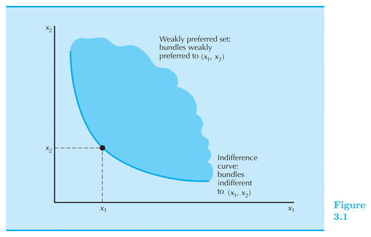
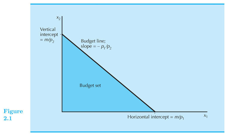
The story so far, in two graphs:


Budget set:
All bundles that cost at most m
Preferred set:
All bundles that are preferred to X
Goal: find most preferred bundle in the budget set.
Remember: the budget set is determined by prices and income;
the preferred set is determined by consumer preferences! DIFFERENT!
Bringing the Budget Set and Preferred Set Together
We now have quantitative descriptions of both the budget set and preferred set.
Topic for today: how do we solve for the optimal bundle?
The Optimization Problem
Utility from bundle X
Cost of Bundle X
Income
Suppose bundle X* solves this problem.
What can we say about the set of preferred bundles to X*?
Insight #1:
If preferences are monotonic, the optimal bundle must lie along the budget line.
The Optimization Problem
If preferences are (strictly) monotonic, the constraint is met with equality.
So the question becomes: what is the highest-utility bundle along the budget line?
Let \(m_1\) be the amount of money spent on good 1
What happens if you spend a little more money on good 1 (move to the right along the budget line)?
What happens if you spend a little more money on good 1 (move to the right along the budget line)?
Suppose apples are good 1 and cost $0.50 each. If you spend one more dollar on apples, how many more do you get?
Suppose bananas are good 2 and cost $0.25 each. If you spend one more dollar on apples, how many fewer bananas do you get?
pollev.com/chrismakler

What happens if you spend a little more money on good 1 (move to the right along the budget line)?
If you spend one more dollar on good 1,
and good 1 costs \(p_1\) per unit,
how much more good 1 do you have?
If you spend one more dollar on good 1,
and good 2 costs \(p_2\) per unit,
how much less good 2 do you have?
Suppose apples are good 1 and cost $0.50 each. If you spend one more dollar on apples, how many more do you get?
Suppose bananas are good 2 and cost $0.25 each. If you spend one more dollar on apples, how many fewer bananas do you get?
What happens if you spend a little more money on good 1 (move to the right along the budget line)?
If you spend one more dollar on good 1,
and good 1 costs \(p_1\) per unit,
how much more good 1 do you have?
If you spend one more dollar on good 1,
and good 2 costs \(p_2\) per unit,
how much less good 2 do you have?
Utility gain from more good 1
Utility loss from
less good 2
What happens if you spend a little more money on good 1 (move to the right along the budget line)?
Utility gain from more good 1
Utility loss from
less good 2
We sometimes call \(MU/p\)
"bang for your buck":
it measures the increase in utility
from spending one more dollar on the good.
Change in utility from spending another dollar on good 1 (moving to the right along the budget line)
Utility gain from more good 1
Utility loss from
less good 2
buying more good 1 increases your utility
buying more good 1 decreases your utility
Review: Slopes, Thus Far
Chapter 2
Budget Constraint
Chapter 3
Preferences
Any slope in Good 1 - Good 2 space is measured in units of good 2/units of good 1.
Chapter 4
Utility
The slope of the indifference curve is the MRS: that is,
the rate at which a consumer is willing to exchange good 2 for good 1.
The slope of the budget line is the price ratio: that is,
the rate at which the market will allow consumers to exchange good 2 for good 1.
What does it mean if the MRS is
greater than the price ratio?
The consumer is more willing to give up good 2
to get good 1
than the market requires.
The consumer receives more utility per additional unit of good 1 than the price reflects, relative to good 2.
The consumer receives more
"bang for the buck"
(utils per dollar)
from good 1 than good 2.
Regardless of how you look at it, the consumer would be
better off moving to the right along the budget line --
i.e., consuming more of good 1 and less of good 2.
Indifference curve is
steeper than the budget line
Indifference curve is
flatter than the budget line
Moving to the right
along the budget line
would increase utility.
Moving to the left
along the budget line
would increase utility.
More willing to give up good 2
than the market requires.
Less willing to give up good 2
than the market requires.
This "gravitational force" is always true.
In certain circumstances, but not always,
this leads us to the tangency condition \(MRS = p_1/p_2\).
At that point, utility is flat as we move along the budget line.
BUY MORE GOOD 1
BUY LESS GOOD 1
Why? If we plot utility along the budget constraint,
\(MRS > p_1/p_2\) means utility is increasing, and \(MRS < p_1/p_2\) means utility is decreasing.
Important and Difficult Distinction
The budget line and indifference curves describe different things.
Indifference curves describe the "shape of the utility hill."
They do not change when prices or income change.
They do change when preferences change, but we usually assume preferences are fixed.
The budget line describes the boundary of affordable bundles;
we can think of it as a fence over the utility hill.
[10 minute break]
“Well-Behaved" Optimality
IF...
THEN...
The consumer's utility function is "well behaved" -- smooth, strictly convex, and strictly monotonic
The indifference curves do not cross the axes
The budget line is a simple straight line
The optimal consumption bundle will be characterized by two equations:
More generally: the optimal bundle may be found using the Lagrange method
How do you tell if a utility function is well behaved and the indifference curves don't cross the axis?
Strictly monotonic
Strictly convex
Smooth
Doesn't cross horizontal axis
Doesn't cross vertical axis
\(MU_1 > 0\) and \(MU_2 > 0\) for any \(x_1,x_2\)
\(\frac{\partial MRS}{\partial x_1} \le 0\) and \(\frac{\partial MRS}{ \partial x_2} \ge 0\), with at least one strict
MRS has no "jumps" (not defined piecewise)
\(MRS=\infty\) whenever \(x_1 = 0\)
\(MRS=0\) whenever \(x_2 = 0\)
The Lagrange Method
Let's rewrite the constraint in the form \(g(x_1,x_2) = 0\)
OBJECTIVE FUNCTION
CONSTRAINT
The Lagrange Method
Income left over
OBJECTIVE FUNCTION
CONSTRAINT
UTILS
$
UTILS
$
What do we want to maximize?
First Order Conditions
"Bang for your buck" condition: marginal utility from last dollar spent on every good must be the same!
First Order Conditions
Cross multiply:
First Order Conditions
TANGENCY CONDITION
CONSTRAINT
The Lagrange method finds the point along the constraint
where the constraint is tangent to a level set of the objective function.
The Lagrange method finds the point along the constraint
where the constraint is tangent to a level set of the objective function.
pollev.com/chrismakler

Utility Function
Budget Constraint
- Write an equation for the tangency condition.
- Solve for \(x_2\) as a function of \(x_1\) (or vice versa).
- Plug that into the budget constraint and solve for \(x_1^*\)
- Plug \(x_1^*\) back into the (2) to solve for \(x_2^*\).
Procedure for Solving a Well-Behaved Optimal Choice Problem
pollev.com/chrismakler

pollev.com/chrismakler

Utility Function
Budget Constraint
- Write an equation for the tangency condition.
- Solve for \(x_2\) as a function of \(x_1\) (or vice versa).
- Plug that into the budget constraint and solve for \(x_1^*\)
- Plug \(x_1^*\) back into the (2) to solve for \(x_2^*\).
Procedure for Solving a Well-Behaved Optimal Choice Problem
Why do we use Lagrange instead of just
plugging the constraint into the utility function?
Conclusions and Next Steps
Bringing preferences and budget sets together, we find the most preferred bundle in a budget set.
Under certain important conditions
(well-behaved utility function, simple straight budget line, indifference curves don't cross the axes)
the optimal consumption bundle will be the point along the budget line
where the consumer's MRS is equal to the price ratio -- i.e., "bang for their buck" is equalized. Mathematically, the Lagrange method finds this point.
Along a budget line, if the MRS is greater than the price ratio,
the consumer gets more "bang for their buck" from good 1 than good 2;
so they can be made better off by choosing more of good 1 and less of good 2; and vice versa.
Next time: look at cases when the optimal bundle is not characterized by a tangency condition.
Econ 50 | 04 | Optimal Choice when Calculus Works
By Chris Makler
Econ 50 | 04 | Optimal Choice when Calculus Works
Comparing MRS and the price ratio; "Gravitational pull" towards optimality; Lagrange method; optimal choice with Cobb-Douglas preferences
- 1,348


