Welcome to Econ 51
To navigate: press "N" to move forward and "P" to move back.
To see an outline, press "ESC". Topics are arranged in columns.
Today's Agenda
Part 1: Course Overview
Part 2: Review of Econ 50
Introductions and Welcome
Three Themes and a Goal
Class Organization and Policies
Unit Overview
Budget sets and Preferences
Constrained Optimization
Specific Utility Functions
Demand and Offer Curves
To Do Before Next Class
Introductions and Welcome
Chris Makler
- B.A.: Humanities, Yale
- Ph.D.: Economics, Penn
(search & matching theory)
- 10 years in the education technology industry
- Sixth time teaching Econ 51
- Office: Landau Econ Building, Room 144
Welcome to Econ 51!

TA Introductions

Sharon

Andy
Econ Department Peer Advising
Other Resources
VPTL Peer Tutoring
Three Themes and a Goal
Theme I: Efficiency and Equity
Why does the market system lead to efficient but
(potentially) inequitable allocations of goods?
Move from looking at bundles of good for a single individual to allocations of goods across individuals.
Under what kinds of circumstances does
everyone solving their own optimization problem
not lead to efficient outcomes?
Theme II: Time
(1) We'll treat "good 1" as "consumption now" and "good 2" as "consumption later" and apply the usual consumer model to "intertemporal choice" models of borrowing and saving.
In Econ 50 we looked only at "static" models in which people were making a decision at a single point in time.
In Econ 51 we'll think of time in two ways:
(2) We'll look at sequential and repeated games, in which players don't move at the same time, but respond to each others' past moves.
Theme III: Information
(1) We'll treat "good 1" as "consumption in one state of the work" and "good 2" as "consumption in another state of the world" and apply the usual consumer model to analyze "risk aversion" and models of insurance and diversification.
In Econ 50 we looked only at "deterministic" models in which everyone had all relevant information about each transaction.
In Econ 51 we'll think of information in two ways:
(2) We'll look at games of incomplete information, when players don't know other players' payoffs or actions.
Overall Goal of the Course:
Refine the Toolset of Econ 50 for More Realistic Applications
Econ 1
Econ 50
Econ 51
Finance
Labor and Education
Public Goods and Optimal Tax
Environmental Economics
Strategic Competition
Auctions and Market Design
Vocabulary
Tools
Refinements
Applied Micro Field Courses
Optimization
Comparative
Statics
Equilibrium
Efficiency
Time
Information
Applications
Micro/Macro
Supply and Demand
Scarcity and Choice
Class Organization
Before Lecture
- Do the reading
- Take online quizzes (easy!)
- 5% of grade
- Graded for correctness, not just completion
Lecture
- Estabish motivation and context
- Work through simple examples
Homework
- Apply concepts from lecture to new situations, more complex examples
- Full credit: earn 100 points in 10 weeks
- 20% of grade
Exams
-
Midterm: Units I & II
(30% of grade) -
Final: Units III & IV
(45% of grade)
[declarative]
[strategic/
schematic]
[procedural]
[cumulative]
Homework Policy
-
Exercises are posted after each lecture, and should be uploaded to Canvas by midnight a few days later. (Tuesday lectures are due Friday night, Thursday lectures are due Monday night.) Solutions are posted at 8am, so homeworks uploaded after 8am are not accepted.
-
Old exam questions are included in each problem set to give you extra practice and help prepare for tests.
-
Each exercise or old exam problem is worth 3-5 points. Your goal is to earn at least 100 pointsfor the quarter (about 10 points per week). Earning beyond 100 points doesn't help your grade, but earning below 100 points will hurt it.
-
Goal: everyone gets 100% homework grade, in the most useful way for them.
Use the problem sets to identify which areas you've got down cold, and which you need more help with. Earn needed points by doing old exam questions on areas you find hard. -
Don't stop when you reach 100 points! Doing exercises is how you learn; people who stop at 100 points tend to do worse on the final by about one letter grade.
Intermediate Microeconomics
by Hal Varian
(Edition is unimportant.)
Strategy
by Joel Watson

No Electronics in Lecture
No phones.
No tablets.
No laptops.
No video or audio recording.
Missing Work
Quizzes
Exercises
Exams
Drop lowest three scores
You just need to earn 100 points over the quarter.
Illness or emergency: contact me before the test starts.
If you do less on one assignment, just do more on another!
Unit Overview
Unit II
The Edgeworth Box and Efficiency
Tuesday 4/30
Midterm on Units I and II
Unit III
Games with Full Information
Unit IV
Bayesian Games and Mechanism Design
Tuesday 6/11
Final Exam on Units III and IV
Course Units (4-5 lectures each)
Unit I
Optimization from an Endowment
[10 minute break]
Sign up for Piazza.
Budget Sets
Good 1 - Good 2 Space
Two "Goods" : Good 1 and Good 2
A "consumption bundle" is a pair of quantities.
\text{Example: Bundle }X\text{ may be written }(x_1,x_2)
x_1 = \text{quantity of good 1 in bundle }X
x_2 = \text{quantity of good 2 in bundle }X
\text{Similarly, bundle }Y\text{ may be written }(y_1,y_2)\text{, etc.}
m = \text{money income}
p_1 = \text{price of good 1}
p_2 = \text{price of good 2}
\text{horizontal intercept} = \frac{m}{p_1}
\text{vertical intercept} = \frac{m}{p_2}
\text{slope of budget line} = -\frac{p_1}{p_2}
Budget Constraint
GOOD 1
GOOD 2
Preferences
Every consumption bundle has a cost.
Given a bundle and prices,
we can divide the choice space
into "more expensive" and
"less expensive bundles.
Given a bundle and preferences,
we can divide the choice space
into "preferred" and
"dispreferred" bundles.
Every consumption bundle has a benefit.
MRS: Slope of the Indifference Curve
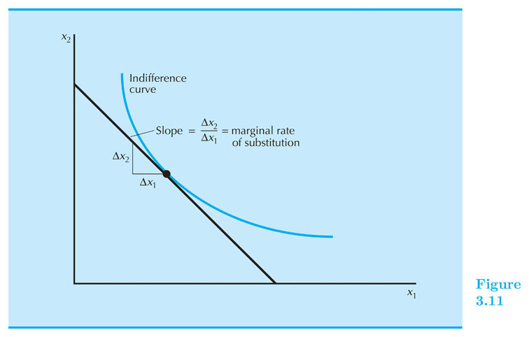
"How many units of good 2 are you willing to give up
to get another unit of good 1?"
"How much good 2 would I need to give you
in order to give up one unit of good 1?"
Or, in the special case where good 1 is "this good"
and good 2 is "dollars spent on other things:"
"How much money (
i.e., units of good 2) would you be willing to pay
for an additional unit of this good (
i.e., good 1)?"
(or equivalently)
The “Gravitational Pull"
Towards Optimality
MRS > \frac{p_1}{p_2}
MRS < \frac{p_1}{p_2}
Indifference curve is
steeper than the budget line
Indifference curve is
flatter than the budget line
Moving to the right
along the budget line
would increase utility.
Moving to the left
along the budget line
would increase utility.
More willing to give up good 2
than the market requires.
Less willing to give up good 2
than the market requires.
GOOD 1
GOOD 2
IF...
THEN...
The consumer's utility function is "well behaved" -- smooth, strictly convex, and strictly monotonic
The indifference curves do not cross the axes
The budget line is a simple straight line
The optimal consumption bundle will be characterized by two equations:
MRS = \frac{p_1}{p_2}
p_1x_1 + p_2x_2 = m
More generally: the optimal bundle may be found using the Lagrange method
- Write an equation for the tangency condition.
- Write an equation for the budget line.
- Solve for x1* or x2*.
- Plug value from (3) into either equation (1) or (2).
Procedure for Solving a Well-Behaved Optimal Choice Problem
When not well-behaved: use logic!
Utility Functions
We'll focus on three "forms" of utility functions:
u(x_1,x_2) = av(x_1) + bv(x_2)
u(x_1,x_2) = v(x_1) + x_2
u(x_1,x_2) = \min\left\{\frac{x_1}{a},\frac{x_2}{b}\right\}
Weighted average of some common "one-good" utility function v(x):
"Quasilinear": one good enters linearly
(in this case \(x_2\)), another nonlinearly:
Perfect complements:
not used as often, but helpful
u(x_1,x_2) = av(x_1) + bv(x_2)
v(x) = \ln x
v(x) = \sqrt{x}
v(x) = x
v(x) = x^2
u(x_1,x_2) = a \ln x_1 + b \ln x_2
u(x_1,x_2) = a \sqrt{x_1} + b\sqrt{x_2}
u(x_1,x_2) = ax_1 + bx_2
u(x_1,x_2) = ax_1^2 + bx_2^2
Cobb-Douglas (decreasing MRS)
Weak Substitutes (decreasing MRS)
Perfect Substitutes (constant MRS)
Concave (increasing MRS)
u(x_1,x_2) = v(x_1) + x_2
Quasilinear
MRS = v'(x_1)
Demand and Offer Curves
(Gross) Demand Functions
Demand Curve for Good 1
x_1^*(p_1,p_2,m)
x_2^*(p_1,p_2,m)
Price Offer Curve for Good 1
\text{Holding }p_2\text{ and }m\text{ constant, plot }(x_1^*(p_1),p_1)\text{ in quantity-price space}
\text{Holding }p_2\text{ and }m\text{ constant, plot }(x_1^*(p_1),x_2^*(p_1))\text{ in Good 1 - Good 2 space}
Demand curves show the functional relationships between price and quantity demanded.
Offer curves show sets of possible endogenous variables.
(Gross) demand functions are mathematical expressions
of endogenous choices as a function of exogenous variables (prices, income).
To Do Before Next Class
Be sure you're signed up for a section.
Do the reading and the quiz -- due at 11:15am on Thursday!
Read the syllabus carefully.
Look over the summary notes for this class.
Econ 51 | 01 | Welcome to Econ 51
By Chris Makler
Econ 51 | 01 | Welcome to Econ 51
Welcome to Econ 51


